Iowa State University Calculus 1
Professor Butler · Iowa State University · 24 lectures with notes
Students in this class: ask your lecturer for the class code, and these lectures will already be in your library when you sign up.
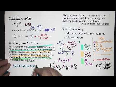
Linearization (but mostly more related rates) (Calc 1; Lecture 2-5; Fall 26)
Related rates turn geometric relationships into equations for unknown speeds, while tangent lines provide local approximations such as √65 ≈ 8.0625.
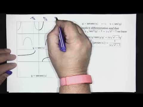
Related rates (Calc 1; Lecture 2-4; Fall 26)
Related rates turns a geometric equation into a relationship between changing quantities, as shown by a sliding ladder and a rising rocket.
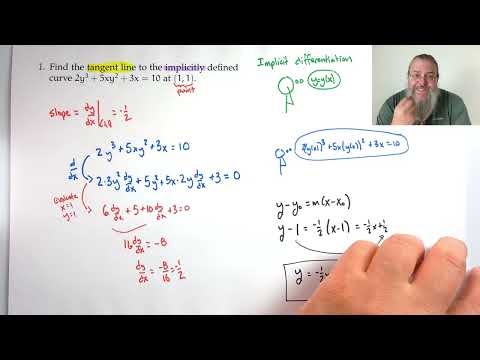
Calc 1 -- Practice for Quiz 5 (Fall 2026)
Beard Meets Calculus solves 10 Quiz 5 problems on implicit derivatives, logarithmic differentiation, inverse functions, and tangent lines.
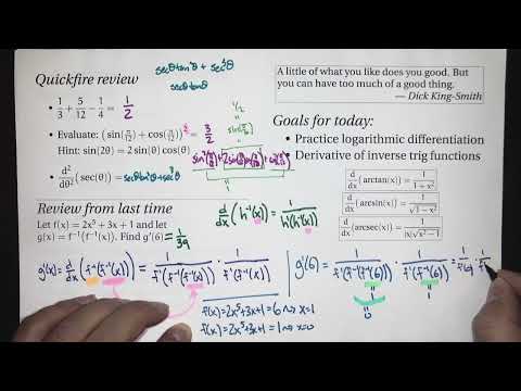
Inverse trigonometric functions (Calc 1; Lecture 2-3; Fall 26)
Derive arctangent and arcsine derivatives, and use logarithms to differentiate variable-exponent functions such as x^x.
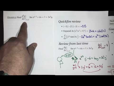
Derivatives of inverses and logs (Calc 1; Lecture 2-2; Fall 26)
Inverse-function derivatives and logarithmic differentiation extend the derivative toolkit through implicit differentiation and log rules.
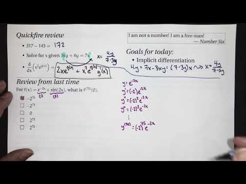
Implicit differentiation (Calc 1; Lecture 2-1; Fall 26)
Implicit differentiation finds dy/dx from an x-y relationship by treating y as a function of x and applying the chain rule.
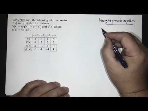
More practice and review (Calc 1; Lecture 1-12; Fall 26)
A Calc 1 exam review focused on applying derivative rules, reading function data, and preparing systematically.
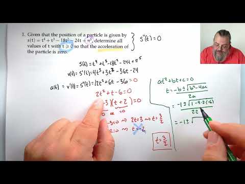
Calc 1 -- Practice for Quiz 4 (Fall 2026)
Ten Calc I practice problems reinforce derivative rules, tangent-line reasoning, differentiability, and graph-based calculations.
Chain rule (Calc 1; Lecture 1-11; Fall 26)
The chain rule differentiates nested functions by multiplying the outside derivative by the inside derivative.
Derivative of trigonometric functions (Calc 1; Lecture 1-10; Fall 26)
Derive and apply the sine, cosine, tangent, and secant derivative rules, including a 137th-derivative pattern.
Derivative as a rate of change (Calc 1; Lecture 1-9; Fall 26)
Derivatives describe change across functions, geometry, units, and motion—from circle growth to a projectile’s 36-foot maximum height.
Calc 1 -- Practice for Quiz 3 (Fall 2026)
Ten Calc 1 practice problems connect derivative rules and limit definitions to tangent-line, perpendicularity, and differentiability questions.
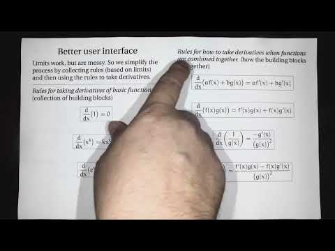
Rules for derivatives (Calc 1; Lecture 1-8; Fall 26)
A practical toolkit for differentiating functions mechanically with power, linearity, product, and quotient rules.
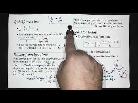
Derivative as a function (Calc 1; Lecture 1-7; Fall 26)
A derivative is a function of tangent slopes, and piecewise differentiability requires both continuity and matching one-sided derivatives.
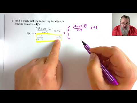
Calc 1 -- Practice for Quiz 2 (Fall 2026)
Ten worked Calc 1 problems show how limit tools and continuity conditions solve common Quiz 2 question types.
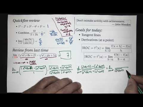
Derivative at a point (Calc 1; Lecture 1-6; Fall 26)
The derivative at a point is the limit of average rates of change and determines the function’s local tangent line.
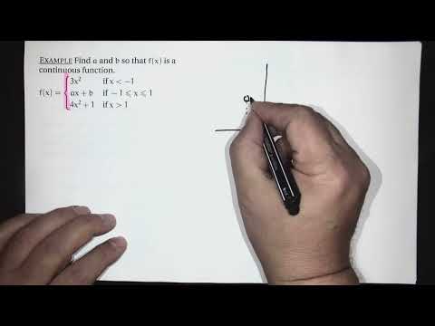
More with continuity; limits with infinity (Calc 1; Lecture 1-5; Fall 26)
Continuity makes many limits direct substitutions, while asymptotes require tracking behavior and signs at infinity or near a zero denominator.
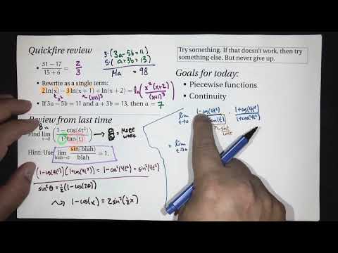
One-sided limits; continuity (Calc 1; Lecture 1-4; Fall 26)
One-sided limits determine whether piecewise functions have limits, while continuity requires the limit and function value to match.
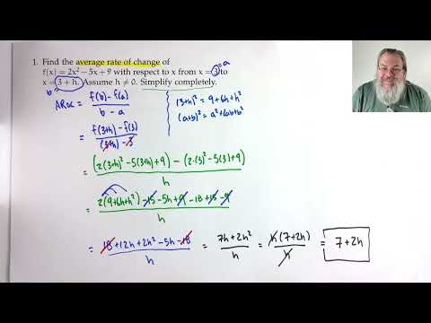
Calc 1 -- Practice for Quiz 1 (Fall 2026)
Ten Calc 1 practice problems show how algebra, one-sided limits, and function composition resolve common Quiz 1 questions.
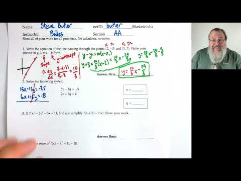
Calc 1 -- Practice Preparation Quiz (Fall 2026)
A worked Calc 1 quiz review covering core algebra, functions, graph shifts, logarithms, and exact trigonometric values.
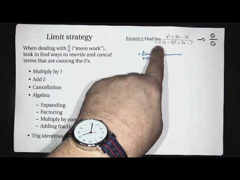
More limits (Calc 1; Lecture 1-3; Fall 26)
Use substitution, algebraic cancellation, and the squeeze principle to evaluate limits, including the foundational radians-based limit sin(θ)/θ → 1.
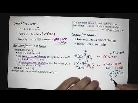
Limits (Calc 1; Lecture 1-2; Fall 26)
Limits describe nearby behavior and let secant slopes approach the tangent slope that defines instantaneous rate of change.
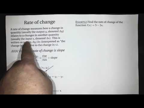
Average rate of change (Calc 1; Lecture 1-1; Fall 26)
Average rate of change is the secant-line slope between two function inputs, calculated as (f(b) − f(a))/(b − a).
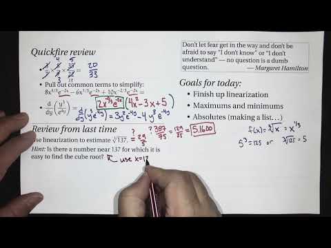
Critical points (Calc 1; Lecture 2-6; Fall 26)
Use tangent lines to estimate function values, then narrow extrema searches to critical points and interval endpoints.