Critical points (Calc 1; Lecture 2-6; Fall 26)

Overview

This Calc 1 lecture connects tangent-line linearization to practical estimates, showing that the cube root of 137 is approximately 5.16 and that an input tolerance of ±0.05 can produce an estimated output tolerance of ±2.4. It then defines absolute and local extrema, uses derivative behavior to identify critical-point candidates, and introduces the Extreme Value Theorem and the candidate-checking method for finding absolute maxima and minima.

Key takeaways

For f(x) = x^(1/3), linearizing at x = 125 estimates ∛137 as 5.16, close to the actual value of about 5.1551.
The linear approximation Δy ≈ f′(a)Δx turns input tolerances into output estimates; for f(x) = 5x³ − 4e^(3x−6) at x = 2, an input tolerance of ±0.05 yields an estimated output tolerance of ±2.4.
A differentiable interior point with nonzero derivative cannot be a local maximum or minimum because small moves in opposite directions produce both larger and smaller values.
Critical points are candidates, not guarantees: x = 0 is a critical point of x³ because its derivative is zero, but x³ has no local extremum there.
A continuous function on a closed, bounded interval is guaranteed to attain absolute extrema; checking critical points and endpoints reduces the search to a finite candidate list.
Under the non-strict definitions of local extrema, every point on a horizontal segment is simultaneously a local maximum and a local minimum.

Chapters

0:00 Quickfire Review: Fraction Cancellation, Factoring, and Derivatives

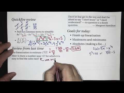
Cancel common factors in the product of 3/7, 8/9, and 35/22 to obtain 20/33.
Factor 2x^(-2/3)e^(-2x) from the expression with x-powers 4/3, 1/3, and -2/3, leaving 4x² − 3x + 5.
Rewrite y³/e^(4y) as y³e^(-4y) and apply the product rule; the derivative is e^(-4y)(3y² − 4y³).

6:45 Linearizing the Cube-Root Function to Estimate ∛137

Choose x = 125 as the nearby reference point because ∛125 = 5.
For f(x) = x^(1/3), use f′(x) = (1/3)x^(-2/3), giving f′(125) = 1/75.
Evaluate the tangent-line approximation L(137) = 5 + (1/75)(137 − 125) = 5.16; the actual value is about 5.1551.

16:17 Margaret Hamilton’s Advice: Ask Questions to Learn

Margaret Hamilton, known for helping program computers used in the Apollo Moon landings, is cited urging students not to let fear prevent questions.
The lecture emphasizes saying “I don’t know” or “I don’t understand” as a practical step toward learning, not a failure.
The stated goals are to finish linearization and begin absolute maximums and minimums.

18:18 Using Linearization to Estimate Output Error Tolerances

Linearization gives f(x) − f(a) ≈ f′(a)(x − a), so an input change Δx produces an estimated output change Δy ≈ f′(a)Δx.
For f(x) = 5x³ − 4e^(3x−6), the reference input a = 2 gives f(2) = 36 and f′(2) = 48.
With x within 0.05 of 2, estimate Δy as 48(0.05) = 2.4, so y is approximately within 36 ± 2.4.

25:55 Differentials dy and Actual Changes Δy

Δy represents the actual change in the function, while dy represents the change predicted by its linearization.
For small input changes near the point of tangency, Δy is approximately dy; this is why differential methods estimate function changes.
The notation dy = f′(x)dx describes the linearized change and should not be confused with the derivative notation dy/dx = f′(x).

28:00 Absolute and Local Extrema: Definitions and Graph Examples

An absolute (global) maximum or minimum is the largest or smallest function value over the entire domain; a local (relative) extremum only compares nearby inputs.
The definitions use ≤ and ≥, allowing a maximum or minimum value to occur at multiple points; an absolute extremum is also local under these definitions.
A graph with a missing endpoint can approach a lowest value without attaining it, so it has no absolute minimum; a horizontal segment consists of points that are both local maxima and local minima.

37:47 Derivative Sign and the Critical-Point Test

A positive derivative indicates the function rises to the right; a negative derivative indicates it falls to the right.
At an interior point where the derivative exists and is nonzero, moving left or right allows the function value to increase or decrease, ruling out a local extremum.
Extrema candidates therefore occur where the derivative is zero, where it is undefined, or at a domain boundary; a critical point is only a candidate, as y = x³ shows at x = 0.

41:33 Finding Critical Points on the Restricted Domain [1, 5]

For f(x) = x^(2/3)e^(-x/3), differentiate with the product rule and factor to get f′(x) = (1/3)e^(-x/3)x^(-1/3)(2 − x).
The exponential factor never vanishes; the derivative is zero at x = 2 and undefined at x = 0.
Because the domain is restricted to [1, 5], x = 0 is excluded; include the boundary points 1 and 5 in the candidate list along with x = 2.

47:27 Extreme Value Theorem and the Candidate-Checking Method

The Extreme Value Theorem guarantees an absolute maximum and minimum when a function is continuous on a closed, bounded interval.
Continuity and a closed, bounded domain are both essential: discontinuities or omitted/unbounded endpoints can prevent the function from attaining an extreme value.
To find absolute extrema, list critical points and interval endpoints, evaluate the original function at each candidate, then select the largest and smallest outputs.

Summary, takeaways, and chapters were generated by AI from the video's transcript and may contain errors. The video belongs to its creator, Beard Meets Calculus.