Texas A&M University STAT 638
Professor Sinha · Texas A&M University · 20 lectures with notes
Students in this class: ask your lecturer for the class code, and these lectures will already be in your library when you sign up.
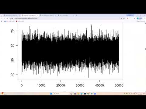
STAT 638 (Fall 2026), Lecture 18
Hierarchical Bayes models share information across groups, and bridge sampling provides a more reliable basis for comparing them than the harmonic-mean estimator.
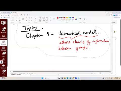
STAT 638 (Fall 2026), Lecture 17
Samiran Sinha derives and implements Gibbs sampling for a Bayesian hierarchical normal model comparing pain thresholds across groups.
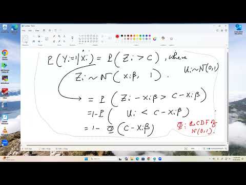
STAT 638 (Fall 2026), Lecture 16
Latent-variable Gibbs sampling makes Bayesian probit regression tractable and leads into hierarchical models for sharing information across groups.
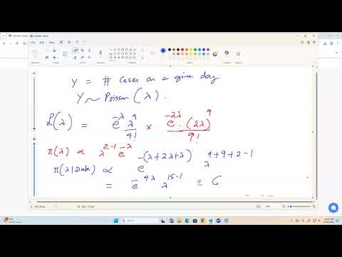
STAT 638 (Fall 2026), Lecture 15
Bayesian quiz solutions connect conjugate updates and mixture posteriors to Monte Carlo uncertainty and prediction.
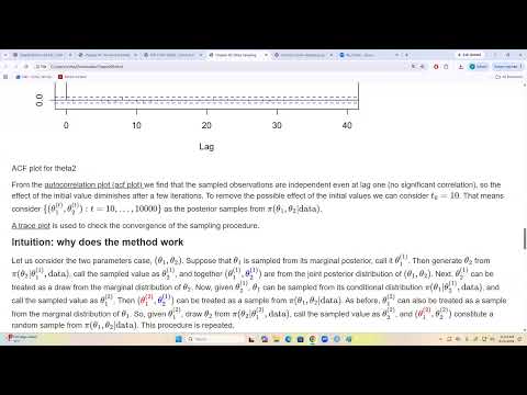
STAT 638 (Fall 2026), Lecture 14
Gibbs sampling turns tractable full conditionals into posterior estimates, with MCMC diagnostics assessing how reliable those estimates are.
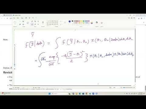
STAT 638 (Fall 2026), Lecture 13
Gibbs sampling builds posterior draws by repeatedly sampling each parameter from its full conditional distribution.
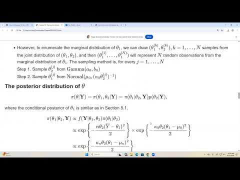
STAT 638 (Fall 2026), Lecture 12
A normal-gamma model and Jeffreys prior turn unknown-mean, unknown-variance inference into posterior sampling and practical summaries.
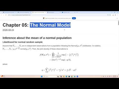
STAT 638 (Fall 2026), Lecture 11
A normal prior yields a normal posterior whose mean combines prior information with the sample mean, while prediction adds observation-level variance.
STAT 638 (Fall 2026), Lecture 10
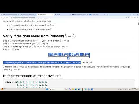
Poisson model checks and Bayes factors show how to assess count-data fit and compare fixed-mean and alternative models.
STAT 638 (Fall 2026), Lecture 9
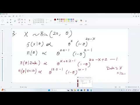
Practice builds the judgment needed to use AI responsibly, while Bayesian examples show how to calculate and simulate posterior predictions.
STAT 638 (Fall 2026), Lecture 8
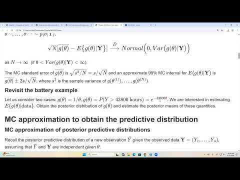
Monte Carlo posterior draws support estimation, prediction, credible intervals, and practical Bayesian model checking.
STAT 638 (Fall 2026), Lecture 7
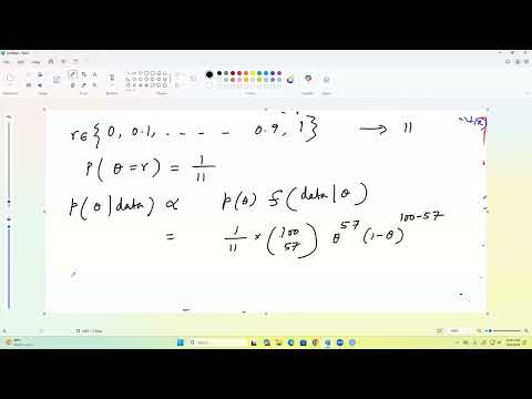
Monte Carlo averages approximate Bayesian posterior summaries without requiring closed-form integration.
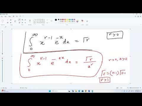
STAT 638 (Fall 2026), Lecture 6
For exponential data, a gamma prior yields a gamma posterior, enabling direct Bayesian inference and prediction.
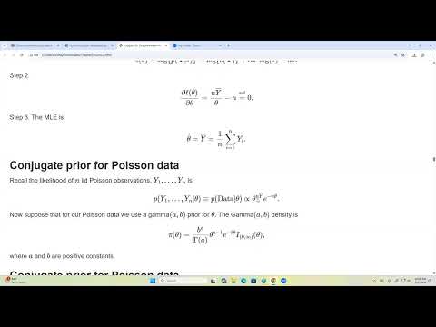
STAT 638 (Fall 2026), Lecture 5
For Poisson counts, Gamma and Jeffreys priors yield tractable posteriors, while mixture priors allow richer Bayesian modeling.
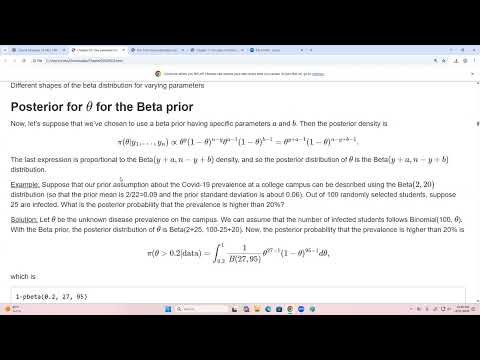
STAT 638 (Fall 2026), Lecture 4
Bayesian estimates combine prior beliefs and data, while prediction and Jeffreys priors address uncertainty and parameterization.
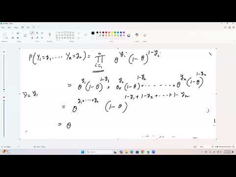
STAT 638 (Fall 2026), Lecture 3
A Beta prior and binomial data give a Beta posterior, making Bayesian inference for a success probability straightforward.
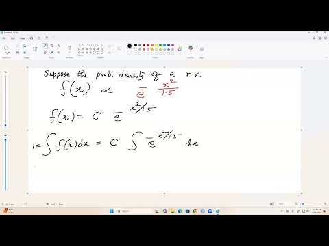
STAT 638 (Fall 2026), Lecture 2
Bayesian inference combines a likelihood with a prior, while exchangeability is weaker than independence.

STAT 638 (Fall 2026), Lecture 1
Samiran Sinha introduces Bayesian inference and demonstrates Bayes’ rule with a diagnostic-testing example.
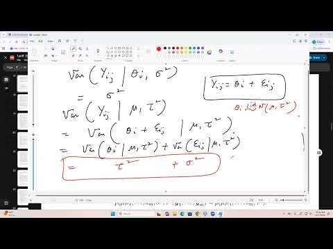
STAT 638 (Fall 2026), Lecture 19
A binomial-beta hierarchical model shares information across hospitals and shrinks uncertain mortality estimates toward the group pattern.
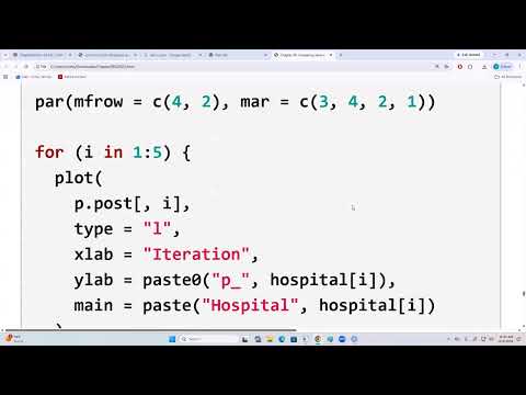
STAT 638 (Fall 2026), Lecture 20
Hospital mortality estimates shrink toward the group mean, while regression connects least squares with Bayesian inference.