STAT 638 (Fall 2026), Lecture 16

Overview

Samiran Sinha develops a Bayesian probit regression for divorce outcomes using age difference as a predictor, then introduces latent-variable data augmentation to make Gibbs sampling practical. He reports a posterior 95% credible interval of 0.103–0.661 for the age coefficient and Pr(β > 0) = 0.999, before introducing hierarchical normal models that share information across groups, illustrated by pain-tolerance scores across four hair-color categories.

Key takeaways

Latent-variable augmentation turns probit regression into a tractable Gibbs sampler by sampling Zᵢ alongside β and C instead of working directly with the integrated observed-data likelihood.
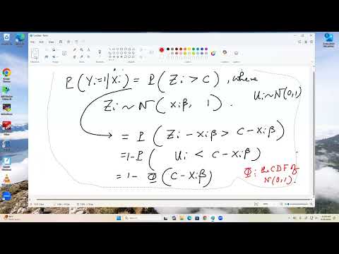
The probit model uses Zᵢ ~ N(Xᵢβ, 1) and classifies divorce as Yᵢ = 1 when Zᵢ > C; the resulting conditional probability is 1 − Φ(C − Xᵢβ).
For the age-difference example, 49,000 retained posterior draws gave a 95% credible interval of 0.103–0.661 and Pr(β > 0) = 0.999, indicating a positive association while leaving conclusions dependent on data coverage.
Hierarchical priors connect group-specific parameters through shared hyperparameters, allowing groups with small samples to borrow information and potentially obtain more stable estimates.
A normal hierarchical model can use normal priors for group means and μ, plus inverse-gamma priors for σ² and τ², yielding convenient Gibbs-sampling conditionals through conjugacy.

Chapters

0:00 Probit Regression for Divorce and Couples’ Age Difference

The example follows 25 married couples over five years and models divorce as a binary outcome.
The predictor is the husband’s age minus the wife’s age; β measures its relationship with divorce probability.
The modeling target is P(Yᵢ = 1 | Xᵢ), where Yᵢ = 1 denotes divorce.

6:30 Deriving the Probit Likelihood and Bayesian Posterior

The latent variable Zᵢ follows N(Xᵢβ, 1), with Yᵢ = 1 when Zᵢ exceeds threshold C.
The success probability is 1 − Φ(C − Xᵢβ), where Φ is the standard normal CDF.
Independent binary observations yield a product Bernoulli likelihood; the posterior combines that likelihood with priors on β and C.

12:00 Why Latent-Variable Augmentation Helps Gibbs Sampling

The observed-data posterior is difficult to evaluate numerically and does not yield convenient full conditional distributions for β and C.
Sinha augments the data with latent Z₁,…,Zₙ, replacing an integrated likelihood with a joint model for observed outcomes and latent variables.
Gibbs sampling can then alternate among β, C, and the Zᵢ values, though each iteration updates N + 2 components.

22:00 Full Conditionals for β, Threshold C, and Latent Zᵢ

Combining the normal likelihood for Zᵢ with the normal prior for β gives a normal full conditional for β, obtained by completing the square.
The outcome indicators constrain C: it must exceed Zᵢ for observations with Yᵢ = 0 and remain below Zᵢ for observations with Yᵢ = 1.
With a normal prior, C has a truncated normal full conditional; each Zᵢ is also normal-truncated above or below C according to its outcome.
Initial values must satisfy the truncation constraints—for example, set C = 1, initialize Zᵢ > 1 when Yᵢ = 1, and Zᵢ < 1 when Yᵢ = 0.

26:00 Diagnosing the Probit Chain and Interpreting Its Posterior

The ACF plots show substantial dependence in β and C, persisting for roughly 40 lags and indicating slow mixing.
Using 49,000 post-burn-in draws after discarding 1,000 iterations, the 95% credible interval for β is 0.103–0.661.
The posterior probability Pr(β > 0) is 0.999, supporting a positive association between the age difference and divorce probability.
Sinha cautions that conclusions about couples with younger husbands depend on whether the data include enough negative age differences.

31:00 Thinning, Code Checks, and the Shift to Hierarchical Models

Thinning is not required to calculate posterior percentiles: Sinha recommends using all retained draws even when autocorrelation is high.
Students can compare their own implementation or code from Claude or ChatGPT with Sinha’s code, checking both results and runtime.
After covering Gibbs sampling in Chapter 6, Sinha postpones Chapter 7’s multivariate normal material and moves to Chapter 8 because hierarchical models support course projects.

35:00 Pain-Tolerance Scores Across Four Hair-Color Groups

The example asks whether pain thresholds differ among light blondes, dark blondes, light brunettes, and dark brunettes.
Pain sensitivity scores summarize individual test performance; a higher score indicates greater pain tolerance.
The table shown contains group summaries, while the hierarchical model is formulated for individual observations within each group.

40:00 Hierarchical Models Borrow Information Across Groups

For group i, individual outcomes Yᵢ₁,…,Yᵢₙᵢ follow a distribution indexed by a group-specific parameter θᵢ.
The group parameters share a distribution π(θ | ψ), and a prior on ψ links the groups through a common hierarchy.
This information sharing can stabilize estimates when group sizes are imbalanced—for example, n₁ = 100, n₂ = 5, n₃ = 4, and n₄ = 20.
Sinha relates hierarchical models to random-effects and mixed-effects models.

45:00 Normal Hierarchy, Conjugate Priors, and Population Means

In the special case, observations within group i are IID normal with population mean θᵢ and a shared within-group variance σ².
The group means have normal priors with common mean μ and variance τ²; σ² and τ² receive inverse-gamma priors, while μ receives a normal prior.
These conjugate choices make Gibbs full conditionals easier to derive, though alternative priors are possible.
The inferential targets are the population means θ₁,…,θₘ and whether they are equal; Bayesian comparisons differ from classical t-tests and ANOVA F-tests.

49:00 Bayesian Inference: From Data and Priors to Posterior Comparisons

The group-mean comparison is framed as H₀: θ₁ = ⋯ = θₘ versus an alternative in which at least one mean differs.
Sinha emphasizes that Bayesian analysis specifies both a data model and prior distributions before drawing posterior conclusions.
The lecture closes with posterior inference for hierarchical group means deferred to the next class.

Summary, takeaways, and chapters were generated by AI from the video's transcript and may contain errors. The video belongs to its creator, Samiran Sinha.