STAT 638 (Fall 2026), Lecture 2

Overview

Samiran Sinha reviews the probability notation and calculations needed for Bayesian inference, derives Bayes’ rule as posterior ∝ likelihood × prior, and explains how prior choice affects posterior conclusions. He distinguishes independence from exchangeability, demonstrates that IID observations are exchangeable but exchangeability alone does not imply independence, then previews Bernoulli and binomial models for Chapter 3.

Key takeaways

Bayesian updating follows π(θ | y) ∝ p(y | θ)π(θ): the posterior’s shape comes from multiplying the data likelihood by the prior, while the marginal likelihood is a θ-independent normalizing constant.
The influence of a prior is most consequential with limited observations; Sinha notes that sufficiently abundant data can reduce, though not necessarily eliminate, prior sensitivity.
Linearity of expectation, E(Y₁ + Y₂) = E(Y₁) + E(Y₂), requires neither independence nor knowledge of the joint distribution.
IID observations are exchangeable because multiplying identical marginal densities is unaffected by reordering, but exchangeability does not by itself establish independence.
In Sinha’s symmetric bivariate example, the marginal is N(0, 1) but the conditional distribution is N(r/2, 0.75); the changing conditional mean shows dependence despite exchangeability.
Conditional IID observations become marginally exchangeable when the shared parameter is integrated out, a property central to Bayesian models of repeated observations.

Chapters

0:00 Quiz Dates and the Chapter 2 Bayesian Foundations

Samiran Sinha lists four quiz dates: September 11, September 25, October 9, and October 23.
The lecture’s groundwork covers probability notation, Bayes’ theorem, posterior distributions, independence, and exchangeability before applying Bayesian methods to models.

2:00 Expectation, Marginalization, and Conditional Distributions

For a discrete random variable, calculate expectation by summing each possible value times its probability; for a continuous variable, replace the sum with an integral.
Obtain a marginal distribution by summing or integrating the joint distribution over the other variable.
A conditional density is the joint density divided by the relevant marginal density, and it sums or integrates to 1.
Linearity gives E(Y₁ + Y₂) = E(Y₁) + E(Y₂) without requiring independence or the joint distribution.

9:15 Proportional Densities and Normalizing Constants

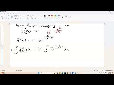
The notation f(x) ∝ g(x) means f(x) = Cg(x) for a constant C.
To make a nonnegative function into a probability density, choose C so its integral over the full domain equals 1.
For a standard normal density, the kernel exp(−y²/2) determines the shape; the proportionality constant supplies normalization.
Sinha uses integration of an exponential quadratic as an example of finding a density’s normalizing constant.

14:35 Bayes’ Theorem: Posterior as Likelihood Times Prior

Let Y be observed data with likelihood p(y | θ), and let π(θ) represent the prior distribution for the unknown parameter θ.
The posterior is π(θ | y) = p(y | θ)π(θ) divided by the marginal data density, found by integrating the numerator over θ.
Because the denominator does not depend on θ, posterior calculations can often use π(θ | y) ∝ p(y | θ)π(θ).
The marginalization integral can be difficult in high-dimensional models, which makes working with the unnormalized posterior useful.

23:19 Prior Choice and the Meaning of Independence

Bayesian posterior distributions depend on the prior: substantially different priors can produce different posteriors.
With sufficient observations, the prior may have moderate or minimal influence; with limited data, its influence can be large.
Events A and B are independent when P(A ∩ B) = P(A)P(B), equivalently when conditioning on B leaves P(A) unchanged.
Mutually exclusive events with positive probabilities are not independent, since learning that one occurred makes the probability of the other zero.

27:48 Conditional Independence and Exchangeability

A and B are conditionally independent given C when P(A ∩ B | C) = P(A | C)P(B | C).
For observations Y₁,…,Yₙ conditionally independent given θ, their joint density given θ factors into the product of their conditional densities.
Bayesian models treat θ as random, so observations are often described as independent conditional on θ.
Exchangeability means the joint distribution is unchanged under any permutation of the observations; for two variables, swapping Y₁ and Y₂ leaves the joint distribution unchanged.

34:44 IID Observations Are Exchangeable, but the Reverse Need Not Hold

If observations are independent and identically distributed, their joint density is a product of identical marginal densities.
Commutativity of multiplication makes that joint density invariant to reordering, so IID observations are exchangeable.
Exchangeability alone does not imply independence; Sinha illustrates this with a symmetric bivariate density proportional to exp[−(c² + r² − cr)/1.5].
For that example, the marginal distribution is N(0, 1), while the conditional distribution of one variable given the other is N(r/2, 0.75), demonstrating dependence despite exchangeability.

42:43 Paper-and-Pencil Practice and Online Assessment

Sinha recommends working through calculations by hand rather than only viewing them on a computer screen.
The course assessment includes online quizzes and an online project; Sinha says students may use tools such as ChatGPT for project help.
He advises students to review and take responsibility for project submissions rather than disguising AI assistance with deliberate typos.

44:38 Conditional IID Sampling Produces Marginal Exchangeability

If Y₁,…,Yₙ are IID conditional on θ, their conditional joint density is a product of identical terms.
Integrating over the shared parameter θ preserves invariance to reordering, so the observations are exchangeable marginally.
For two observations, swapping values r and s leaves the integrated joint distribution unchanged.

47:00 Chapter 3 Preview: Bernoulli and Binomial Models

Chapter 3 begins Bayesian inference for one-parameter models, including Bernoulli, binomial, and Poisson models.
A Bernoulli variable takes value 1 for success with probability π and 0 for failure with probability 1 − π.
A binomial experiment consists of independent, identically distributed Bernoulli trials with the same success probability.
Sinha introduces glossophobia as an example: randomly selecting a student and recording whether that student has fear of public speaking creates a Bernoulli outcome.

Summary, takeaways, and chapters were generated by AI from the video's transcript and may contain errors. The video belongs to its creator, Samiran Sinha.