STAT 638 (Fall 2026), Lecture 9

Overview

Samiran Sinha emphasizes that learning STAT 638 requires working problems by hand, even when AI can produce answers, and demonstrates Bayesian inference through binomial and Poisson examples. The lecture derives posteriors and credible intervals, calculates a Jeffreys-prior marginal likelihood while checking an AI-generated numerical result, and shows how to simulate posterior predictive observations for a Poisson model.

Key takeaways

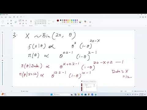
A Beta(0.2, 2) prior updated with 12 successes and 8 failures gives a Beta(12.2, 10) posterior, with a reported median of 0.5511 and 95% credible interval of approximately 0.344–0.745.
For 12 successes in 20 trials, the Jeffreys prior is Beta(0.5, 0.5), producing a Beta(12.5, 8.5) posterior and a reported 95% credible interval of approximately 0.38–0.789.
The Jeffreys-prior marginal likelihood for the observed binomial count is C(20,12) × B(12.5,8.5) / B(0.5,0.5), approximately 0.031; retaining the prior's normalization constant is essential.
With λ | data distributed as Gamma(12, rate 4), the predictive probability of zero Poisson events is E[e^−λ | data], approximately 0.068 by Monte Carlo averaging.
For Poisson data with a Gamma(2, rate 1) prior, conjugacy gives a Gamma(2 + ΣYi, n + 1) posterior; posterior predictive simulation alternates a parameter draw and a Poisson count draw.

Chapters

0:00 Why Completing STAT 638 Homework Matters More Than Easy Grades

Samiran Sinha says auditing a course without assignments left him with little learning, despite attending lectures.
He argues that AI may help students obtain correct answers or grades without building the statistical judgment needed for real problems.
Students who have fallen behind should treat today as the first day and begin practicing the posted homework problems and solutions.

4:54 Posterior Predictive Distributions Require Conditional Independence

For a new observation Ỹ, Sinha writes its predictive density as an integral over the parameter posterior.
The simplification to integrating f(Ỹ | θ) times π(θ | data) relies on Ỹ being conditionally independent of the observed data given θ.
The independence assumption is appropriate for a new, independent patient or observation under the sampling model.

6:27 Beta-Binomial Update for 12 Successes Among 20 Patients

With 12 successes in 20 patients and a Beta(0.2, 2) prior, conjugacy gives a Beta(12.2, 10) posterior for the success probability.
Sinha estimates the posterior median by drawing posterior samples; the reported median is 0.5511.
The reported 95% posterior credible interval is approximately 0.344 to 0.745, using the 2.5th and 97.5th percentiles.

11:40 AI Can Extend Statistical Knowledge but Cannot Replace Its Foundations

Sinha says that knowing statistical basics enables people to use AI to extend their knowledge and apply methods to harder problems.
Without foundational knowledge, students may lack the judgment to choose or assess an appropriate method.
He introduces the Jeffreys prior for a binomial success probability as Beta(0.5, 0.5).

15:51 Deriving the Binomial Jeffreys Prior and Credible Interval

Starting from the binomial log-likelihood, Sinha derives the Fisher information as 20/[θ(1−θ)] for n = 20.
Taking the square root of the information gives a prior proportional to θ^−1/2(1−θ)^−1/2, or Beta(0.5, 0.5).
With 12 successes and 8 failures, the posterior is Beta(12.5, 8.5); the reported 95% credible interval is about 0.38 to 0.789.

21:45 Jeffreys-Prior Marginal Likelihood and Checking AI Arithmetic

For 12 successes out of 20 under a Beta(0.5, 0.5) prior, the marginal likelihood is C(20,12) × B(12.5, 8.5) / B(0.5, 0.5).
The beta-function normalization constant must be retained when computing the marginal likelihood, even though constants independent of θ can be omitted when deriving a posterior.
Sinha verifies the numerical result of about 0.031 in R after an AI-generated calculation produced a conflicting value, underscoring the need to check computation.

32:21 Gamma-Poisson Posterior Predictive Probability of Zero Attacks

For migraine counts modeled as Poisson(λ), the posterior is Gamma(shape 12, rate 4).
The predictive probability of zero attacks is E[e^−λ | data], integrating over the Gamma posterior.
Monte Carlo estimation draws λ values from Gamma(12, 4), evaluates e^−λ for each draw, and averages them; Sinha reports approximately 0.068.

40:29 Restarting Homework Practice with Problems 2.1, 4.1, and 4.2

Sinha recommends starting with Homework 2.1 because the early problems are accessible and can build confidence.
He directs students to the posted solutions, which may need to be opened in a browser.
Because Chapter 4 has been covered, he expects students to attempt problems 4.1 and 4.2 and introduces problem 4.8.

42:53 Poisson-Gamma Conjugacy for Comparing Two Groups’ Child Counts

Problem 4.8 compares average numbers of children for men in their 30s with and without a bachelor's degree, using two data files from the Bayesian analysis book's exercise-data page.
For Poisson observations and a Gamma(2, 1) prior, the posterior for θ is Gamma(2 + ΣYi, n + 1), using the rate parameterization.
The likelihood's factors involving individual factorials can be omitted when deriving the posterior because they do not depend on θ.

48:14 Generate 5,000 Posterior Predictive Counts in Two Steps

To sample from the posterior predictive distribution, first draw θ from its posterior given the observed counts.
Next, draw a new count Ỹ from a Poisson distribution using that sampled θ.
Repeat both steps 5,000 times for each education group, then compare the resulting predictive samples.

Summary, takeaways, and chapters were generated by AI from the video's transcript and may contain errors. The video belongs to its creator, Samiran Sinha.