STAT 638 (Fall 2026), Lecture 6

Overview

Samiran Sinha develops Bayesian inference for an exponential model, moving from its rate parameterization and gamma-function calculations to likelihoods, conjugate and Jeffreys priors, and posterior prediction. He applies the methods to smartphone battery lifetimes, then distinguishes posterior predictive intervals from parameter credible intervals and highest posterior density (HPD) regions; the lecture closes with guidance that the upcoming quiz may include calculations but no proofs.

Key takeaways

For independent observations from an exponential distribution with rate θ, the likelihood depends on the data through the sample mean ȳ, which is sufficient for θ.
A Gamma(A, B) shape-rate prior is conjugate: after n observations with sample mean ȳ, the posterior is Gamma(A+n, B+nȳ).
Jeffreys prior for the exponential rate is proportional to 1/θ; although improper, it produces a proper Gamma(n, nȳ) posterior when n observations are available.
Posterior predictive inference integrates uncertainty in θ rather than substituting a single estimate, so it answers questions about future observations conditional on existing data.
A central credible interval is defined by posterior quantiles, while an HPD interval selects the highest-density region and is typically shorter for a unimodal posterior.
The lecture’s exponential battery model is an assumption, not a universal rule: Sinha notes that Weibull or mixture models may be more appropriate for some lifetime data.

Chapters

0:00 Course Updates, Lecture Plan, and the Value of Written Practice

Samiran Sinha says the class no longer has a TA and asks students to contact him for help.
The planned topics are the exponential distribution, likelihood and priors, posterior prediction, Bayesian intervals, and possibly Monte Carlo methods.
Sinha emphasizes writing out calculations and derivations as essential practice for learning.

2:50 Exponential Density, Rate Parameter, and Gamma Integrals

The exponential density is f(y|θ) = θe^(−θy) for y > 0 and θ > 0; θ is the rate.
Under the rate parameterization, the mean is 1/θ and the variance is 1/θ²; the scale parameterization instead has mean θ and variance θ².
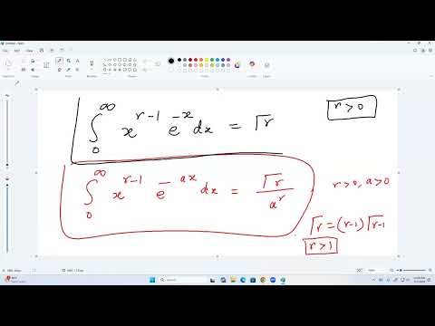
Sinha derives the mean using the gamma integral and reviews Γ(r) = ∫₀∞ x^(r−1)e^(−x)dx and Γ(r) = (r−1)Γ(r−1).

9:00 Exponential Models for Waiting Times and Lifetimes

A positive continuous waiting time, such as the number of days travelers buy domestic airline tickets in advance, can be modeled exponentially; the example mean is 18 days.
If cars pass a highway point according to a Poisson process at 10 cars per minute, the time between successive cars is exponential with mean 0.1 minute, or 6 seconds.
Other inter-arrival examples include ships reaching a port and customers arriving at a bank; battery lifetime is another possible application, though alternatives such as Weibull models may fit better.

13:20 Exponential Likelihood and Gamma Conjugate Posterior

For n independent exponential observations, the likelihood is proportional to θⁿ exp(−nθȳ), where ȳ is the sample mean and is sufficient for θ.
A Gamma(A, B) prior in shape-rate form has kernel θ^(A−1)e^(−Bθ); combining it with the likelihood gives a Gamma(A+n, B+nȳ) posterior.
The posterior mean is (A+n)/(B+nȳ); as n grows, it approaches 1/ȳ, the maximum likelihood estimate of θ.

19:50 Nonconjugate Lognormal Prior and Jeffreys Prior

A lognormal prior for θ generally produces a posterior without a familiar closed-form distribution, so posterior expectations may require numerical methods.
For the exponential likelihood, the Fisher information is n/θ²; Jeffreys prior is therefore proportional to 1/θ.
The Jeffreys prior is improper on (0, ∞), but with n observations it yields a proper Gamma(n, nȳ) posterior whose mean is 1/ȳ.

28:00 Smartphone Battery Data and Jeffreys-Posterior Estimates

Sinha analyzes 10 smartphone battery lifetimes under an exponential model with unknown rate θ and Jeffreys prior 1/θ.
The sample mean is reported as 35,594 hours, approximately 4.06 years; the resulting posterior is Gamma(10, 10 × 35,594) in shape-rate form.
The posterior mean is 1/ȳ, and the posterior standard deviation follows from the Gamma variance formula, shape divided by rate squared.

33:30 Posterior Prediction for a Battery Lifetime Above 25,000 Hours

The posterior predictive probability averages P(Ynew > 25,000 | θ) over the posterior distribution of θ rather than fixing θ at one estimate.
For an exponential observation, the conditional survival probability is exp(−25,000θ); integrating it against the Gamma(10, 10ȳ) posterior gives the predictive probability.
The lecture reports a predictive probability of 0.488 and a plug-in estimate using the posterior mean of 0.495 for this threshold.

37:20 Posterior Predictive Density and Future-Observation Intervals

The posterior predictive density integrates the exponential density for a new observation over the posterior distribution of θ.
With a Gamma(A+n, B+nȳ) posterior, the predictive density has the form k r^k/(r+y)^(k+1), where k = A+n and r = B+nȳ.
A 95% posterior predictive interval uses the 2.5th and 97.5th percentiles of the predictive distribution; it describes uncertainty about a future observation, not θ.
Conjugacy makes the predictive calculation available in closed form, while nonconjugate priors may require numerical integration.

43:30 Bayesian Credible Intervals and Highest Posterior Density Regions

A 100(1−α)% credible region contains at least posterior probability 1−α for θ given the observed data.
A central 95% credible interval uses the posterior 2.5th and 97.5th percentiles; these endpoints differ conceptually from classical confidence limits.
An HPD region has equal posterior density at its endpoints and, for a unimodal density, gives the shortest interval containing the specified posterior probability.
Unlike a central percentile interval, an HPD interval is found by searching for suitable endpoints; Sinha points to the R package HDInterval and its hdi() function.

49:10 Lecture Wrap-Up and Quiz Expectations

Sinha encourages students to begin their projects and practice the lecture calculations over the holiday Monday.
The upcoming quiz is scheduled for the following Friday.
The quiz may include numerical calculations but will not include proofs or derivations.

Summary, takeaways, and chapters were generated by AI from the video's transcript and may contain errors. The video belongs to its creator, Samiran Sinha.