STAT 638 (Fall 2026), Lecture 11

Overview

Samiran Sinha reviews Bayesian model selection for Poisson and negative binomial count models, then develops Bayesian inference for a normal mean with known variance. He derives the normal–normal posterior and predictive distribution, compares Bayesian and frequentist uncertainty, and introduces nuisance parameters for the case where both normal parameters are unknown.

Key takeaways

For the Poisson-versus-negative-binomial example, the Poisson-to-negative-binomial Bayes factor is about 4.91 from marginal likelihoods and 6.32 from the BIC approximation; both favor Poisson among the two candidates.
When σ² is known and μ has prior N(μ₀, σ₀²), the posterior is normal with precision 1/σ₀² + n/σ² and a mean weighted between μ₀ and the sample mean ȳ.
The posterior predictive variance for a new normal observation is σₙ² + σ², combining uncertainty about μ with the variance of the new observation itself.
Bayesian posterior uncertainty conditional on observed data and frequentist sampling variability answer different questions, so comparing their interval widths alone does not establish which method is better.
Realistic simulation studies with known data-generating conditions can assess whether competing methods capture uncertainty adequately; a single observed dataset cannot reveal the truth by itself.

Chapters

0:00 Negative Binomial Parameters, MCMC, and Bridge Sampling

The negative binomial model has a mean parameter μ and a positive shape parameter ω, unlike the one-parameter Poisson model.
Because the likelihood lacks a convenient conjugate prior for both parameters, posterior computation uses MCMC; the lecture identifies the sampler as NUTS and describes priors on log μ and ω.
Bridge sampling estimates log marginal likelihood for the negative binomial model at about −70.37.

6:30 Poisson-versus-Negative-Binomial Bayes Factors and BIC

The Poisson model's log marginal likelihood is about −68.788, yielding a Poisson-to-negative-binomial Bayes factor of roughly 4.91 and strong comparative evidence for Poisson.
A Bayes factor compares candidate models; it does not establish that either model generated the data.
For finite-dimensional models, BIC provides a Laplace-approximation-based estimate of −2 times the log marginal likelihood; the example's BIC approximation gives a Bayes factor of 6.32.
BIC is less suitable when model dimension is unclear, such as in some sparse or regularized models, and Bayesian calculations require a likelihood and prior.

13:00 Normal-Model Likelihood and Sufficient Statistics

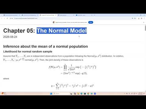
The normal-model section assumes independent observations Y₁,…,Yₙ from N(μ, σ²), with joint likelihood formed as a product because the observations are IID.
The likelihood can be expressed using the sample mean and sample variance; these are sufficient statistics for μ and σ² in the normal family.
Spatial and time-series observations may not be independent, so their likelihoods cannot generally be written as the same IID product.

18:00 Normal Prior and Completing the Square for μ

With σ² known, Sinha assigns μ a conjugate prior N(μ₀, σ₀²), making the posterior calculation tractable.
Multiplying the likelihood kernel by the prior kernel and completing the square gives a normal posterior with precision A = n/σ² + 1/σ₀².
The posterior variance is 1/A, and its mean is B/A, where B = nȳ/σ² + μ₀/σ₀².

24:00 Posterior Mean as a Weighted Average and Large-Sample Behavior

The posterior mean combines the prior mean μ₀ and sample mean ȳ, with weights determined by prior and sampling precision.
As sample size n grows, the data receive increasing weight, the prior's influence diminishes, and the posterior mean approaches ȳ.
Sinha distinguishes Bayesian uncertainty about μ conditional on observed data from the classical sampling distribution, where μ is fixed and ȳ varies.

30:00 Posterior Predictive Distribution for a Future Normal Observation

A future observation is represented as Ỹ = μ + ε̃, where ε̃ is an independent N(0, σ²) observation error.
Combining that error with the posterior μ distribution gives Ỹ conditional on the data a normal distribution with mean μₙ and variance σₙ² + σ².
The predictive variance exceeds the posterior variance of μ because it includes both parameter uncertainty and new-observation noise.

35:00 Ball-Bearing Example and Posterior versus MLE Variance

The example uses 12 ball-bearing diameter measurements and a known process standard deviation of 0.01 cm to infer the process mean.
Computing the posterior requires choosing prior hyperparameters μ₀ and σ₀² in addition to the sample mean and known σ².
With a proper normal prior, posterior variance 1/(1/σ₀² + n/σ²) is smaller than the MLE's sampling variance σ²/n.

42:00 Comparing Bayesian and Frequentist Predictive Uncertainty

A frequentist plug-in prediction replaces μ with the MLE ȳ, producing predictive variance σ²/n + σ².
The Bayesian predictive variance is σₙ² + σ²; its parameter-uncertainty component is smaller than σ²/n in this known-variance, normal-prior example.
The two uncertainty measures are not directly equivalent: the Bayesian predictive distribution conditions on observed data, whereas the frequentist expression involves the unknown fixed μ.

46:00 Why Comparing Interval Widths Requires Simulation

A Bayesian model with more parameters may report greater uncertainty than a more restricted frequentist model, but greater variability is not automatically worse.
Narrow intervals can understate uncertainty if a method omits important variables or sources of variation.
Sinha recommends realistic simulation studies with known data-generating truth to compare methods' uncertainty estimates; one dataset alone is insufficient.

49:00 Introducing Interest and Nuisance Parameters in the Normal Model

The next case treats both normal parameters as unknown and distinguishes a parameter of interest from nuisance parameters.
Sinha parameterizes the normal model with mean θ₁ and precision θ₂, so the variance is 1/θ₂.
The parameter space is ℝ × ℝ⁺, and its constraints guide the choice of priors for subsequent inference.

Summary, takeaways, and chapters were generated by AI from the video's transcript and may contain errors. The video belongs to its creator, Samiran Sinha.