STAT 638 (Fall 2026), Lecture 14

Overview

Samiran Sinha develops Chapter 6’s Gibbs-sampling workflow, from a normal mean–precision example through practical MCMC diagnostics, including autocorrelation, trace plots, effective sample size, burn-in, and thinning. He then derives prior dependence and full conditional distributions for a Poisson comparison of child counts between two groups, and illustrates how Gibbs draws estimate the posterior difference in group rates.

Key takeaways

Gibbs sampling requires tractable full conditional distributions rather than a direct draw from the joint posterior; in the normal example, the updates are normal for θ₁ and gamma for θ₂.
Trace plots and autocorrelation plots diagnose different MCMC issues: trends or stalls suggest convergence or mixing problems, while high lag autocorrelation indicates dependent draws.
Effective sample size translates correlated MCMC output into an independent-draw equivalent; the normal example produces ESS near 10,000 for θ₁ and about 9,252 for θ₂.
Burn-in can reduce sensitivity to initial values, but thinning is usually unnecessary when storage allows retaining all post-burn-in draws.
In the Poisson comparison, θ_A = θ and θ_B = θγ are dependent under the induced prior, even when θ and γ receive separate gamma priors.
For the child-count example, Gibbs draws estimate θ_B − θ at about 0.389, with a reported 95% credible interval of approximately 0.109–0.6427.

Chapters

0:00 Normal Mean–Precision Gibbs Sampling: Model, Priors, and Updates

The example models observations as normal with population mean θ₁ and precision θ₂, using conjugate normal and gamma priors.
The example sets μ₀ = 50, κ₀ = 0.5, a₀ = 0.1, and b₀ = 0.1, and initializes θ₁ = 0 and θ₂ = 10.
Each Gibbs iteration draws θ₁ from its normal full conditional, then θ₂ from its gamma full conditional, whose rate depends on the updated θ₁.
The demonstrated chain stores 10,000 iterations of both parameters.

6:00 Autocorrelation Plots and the Effect of Starting Values

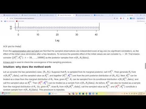
Sample autocorrelation plots for θ₁ and θ₂ show negligible correlations across lags in the normal-model example.
Lag-1 autocorrelation compares consecutive draws; higher lags compare draws separated by that many iterations.
The plotted reference bounds are approximately ±1.96 divided by the square root of the iteration count.
Low autocorrelation suggests limited dependence on initial values after the chain gets underway; discarding early draws, such as the first 10 here, can further reduce that influence.

12:00 Trace Plots, the Markov Property, and Posterior Convergence

A useful trace plot fluctuates around a stable value without sustained trends, long stalls, or visible patterns.
Gibbs draws form a Markov chain: the next parameter state depends on the current state, not the full history.
Under mild regularity conditions, the chain converges to the target posterior distribution.
Posterior probabilities can be estimated by the fraction of retained draws in a set, and posterior expectations by Monte Carlo averages.

17:00 Convergence and Mixing Diagnostics: Chains, ACF, and ESS

Convergence describes approach to the target distribution; mixing describes how efficiently the chain explores parameter space once there.
Comparing multiple chains from different starting values strengthens evidence for convergence when the chains overlap and explore similar regions.
High autocorrelation indicates slow mixing, while low autocorrelation suggests successive draws explore the parameter space more efficiently.
Effective sample size estimates the independent-draw equivalent of correlated MCMC output; the lecture gives ESS = M / (1 + 2Σρₖ), where M is the iteration count and ρₖ is lag-k autocorrelation.

25:00 Burn-In and Thinning: Which MCMC Draws to Retain

Burn-in discards early draws to limit the effect of starting values; the appropriate amount depends on the model and chain behavior.
Many R packages discard an initial portion of iterations, often about half by default, before posterior inference.
Thinning keeps every Lth draw to reduce dependence when approximately independent samples are needed.
When storage is not a constraint, retaining all post-burn-in draws is generally preferable to thinning and discarding useful samples.

28:00 Chapter 6 Practice Problems and Accessing the Notation-Correct PDF

Sinha identifies Chapter 6 homework problems 6.1 and 6.3 and provides solutions for ungraded practice.
Some mathematical notation disappeared when the exercise file was converted for Canvas accessibility.
A Google Drive PDF preserves the original notation and requires a TAMU NetID login for access.
Problem 6.1 is worked through in this lecture; problem 6.3 is left for the next lecture.

31:00 Poisson Child-Count Comparison and Dependence of Group Rates

Problem 6.1 reuses Exercise 4.8 data on numbers of children for men in their 30s, comparing groups with and without a bachelor’s degree.
The group Poisson means are parameterized as θ_A = θ and θ_B = θγ, making γ the relative rate θ_B / θ_A.
Although θ and γ have separate gamma priors, θ_A and θ_B are dependent under the induced prior because both involve θ.
A change-of-variables calculation uses the Jacobian determinant 1/θ_A; the resulting joint density does not factor into separate functions of θ_A and θ_B.

36:00 Deriving Gamma Full Conditionals for the Two-Group Poisson Model

The data contribute 54 and 305 total child counts for groups A and B, with 58 and 218 observations, respectively.
Conditioning on γ, θ has a gamma full conditional with shape 359 + Aθ and rate 58 + 218γ + Bθ.
Conditioning on θ, γ has a gamma full conditional with shape 305 + C and rate 218θ + D.
The requested conditional distributions follow by collecting the likelihood and prior terms involving the parameter being updated.

41:00 Coding Gibbs Updates Across Relative-Rate Prior Choices

The exercise fixes Aθ = 2 and Bθ = 1, then varies the gamma prior parameters C and D together across values including 8, 16, 32, 64, and 128.
For each prior setting, the algorithm alternates draws of θ and γ from their gamma full conditionals and stores the iterations.
The initial values shown are θ = 0.5 and γ = 0.5; the code example runs the sampling loop and calculates θ_A = θ and θ_B = θγ.
Sinha notes that the exercise asks for at least 5,000 iterations and illustrates the calculation using a longer run.

46:00 Posterior Rate Difference and a 95% Credible Interval

For the illustrative prior setting, posterior draws are transformed into θ_B − θ_A = θγ − θ.
The estimated posterior mean difference is about 0.389, close to the provided solution’s value; Monte Carlo estimates can vary across runs.
A 95% credible interval is computed from the 2.5th and 97.5th percentiles of the sampled rate differences.
The reported interval is approximately 0.109 to 0.6427, and the lecture notes that the calculation uses 100,000 Gibbs draws.

Summary, takeaways, and chapters were generated by AI from the video's transcript and may contain errors. The video belongs to its creator, Samiran Sinha.