STAT 638 (Fall 2026), Lecture 18

Overview

Samiran Sinha develops Chapter 8’s Bayesian hierarchical analysis of pain-tolerance data across four hair-color groups, explaining Gibbs-sampling diagnostics, effective sample size, and how group means share information through hyperparameters. He compares equal-means and varying-means models using Bayes factors, contrasts the unstable harmonic-mean estimator with bridge sampling, then extends the model to unequal group variances and reviews classical ANOVA assumptions and practice.

Key takeaways

In the four-group pain-tolerance model, τ² determines the amount of partial pooling: very large τ² leaves group means close to their own data, while τ² near zero pulls them toward a shared mean.
A 50,000-iteration Gibbs chain with 5,000 burn-in draws leaves 45,000 draws for summaries, but autocorrelation means its effective sample size can be much lower than 45,000.
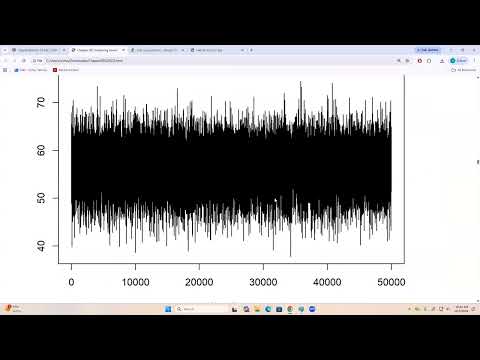
Trace plots reveal chain behavior: a stable band suggests adequate exploration, while prolonged residence in separate regions signals poor mixing and possible sampling problems.
Bayes factors compare models through marginal likelihoods, but prior-based Monte Carlo integration may miss high-density regions and the harmonic-mean estimator can be dominated by extreme inverse-likelihood values.
Bridge sampling combines samples from a proposal distribution and the posterior; in Sinha’s example its log marginal likelihoods of approximately −55 for the null and −50 for the alternative favor unequal group means.
A Bayesian variance hierarchy can model different σᵢ² values while sharing information across groups; the nonstandard conditional for ν₀ may require Metropolis sampling, unlike the standard conditional updates.

Chapters

0:00 Chapter 8, Assessment Topics, and Learning Beyond AI Answers

Sinha previews Chapter 8 and mentions a Friday assessment covering Monte Carlo integration, the normal distribution, and hierarchical models.
He notes that students in STAT 415 often scored 100 on open-internet quizzes but struggled with the same questions on exams.
Sinha encourages students to use AI to check or compare their work, while still learning to solve the problems independently.

2:16 Four-Group Gibbs Sampling: Burn-In, Trace Plots, and Effective Sample Size

The example models pain tolerance across four hair-color groups, with group means θ₁–θ₄, shared mean μ, observation variance σ², and between-group variance τ².
Sinha ran 50,000 Gibbs iterations and discarded 5,000 as burn-in to reduce the effect of arbitrary initial values; the burn-in length should be judged rather than treated as a fixed rule.
A converged trace plot should form a stable band; long stays in separate regions signal poor mixing, which can arise when sampling from nonstandard conditional distributions.
Because MCMC draws are autocorrelated, the time-series standard error accounts for dependence, and effective sample size summarizes how many independent draws the chain approximately provides.

14:53 Partial Pooling: How τ² Shares Information Across Group Means

Each full conditional for θᵢ combines the group sample mean with the shared hypermean μ, which depends on information from all four groups.
The variance τ² controls pooling: as τ² grows very large, group estimates approach their separate group means; as τ² approaches zero, the θᵢ values converge toward a common mean.
Because τ² is estimated from the data, the degree of information sharing is learned rather than fixed in advance.

18:33 Equal-Means Model as the Null Hypothesis

Sinha defines a null model in which θ₁, θ₂, θ₃, and θ₄ are all replaced by one common θ, corresponding to equal underlying group means.
The alternative model retains distinct group means, making the comparison analogous to testing equality of means in ANOVA.
The equal-means model has one θ parameter; its Gibbs sampler also updates σ², τ², and μ from their full conditional distributions.

23:36 Bayes Factors and the Challenge of Marginal Likelihoods

The Bayes factor compares the null and alternative models through the ratio of their marginal likelihoods.
Sinha gives the usual interpretation: a Bayes factor above 3 favors the null substantially, while a value below one-third favors the alternative substantially.
Each marginal likelihood integrates the joint data likelihood over a multidimensional parameter space, including parameters with unbounded ranges, so direct calculation is difficult.
Drawing independently from the prior for simple Monte Carlo integration can miss the high-likelihood regions that matter most to the posterior.

28:37 Why the Harmonic-Mean Marginal Likelihood Estimator Is Unstable

The harmonic-mean method uses posterior samples to estimate the inverse marginal likelihood from inverse likelihood values.
When a sampled parameter value yields a very small data likelihood, taking its inverse creates an extreme value that can dominate the estimate.
Sinha’s example favors the alternative model, but he cautions that harmonic-mean estimates can have high variability and should not be trusted as a robust comparison.

33:00 Bridge Sampling for More Reliable Model Comparison

Bridge sampling estimates the marginal likelihood using Monte Carlo averages from both a proposal distribution and the posterior distribution.
Its bridge function links those two distributions; an optimal choice depends on unknown quantities and is found iteratively.
Sinha recommends the R bridge sampling package and reports log marginal likelihoods of about −55 for the null model and −50 for the alternative.
The alternative’s higher marginal likelihood supports it for this dataset, and Sinha prefers bridge sampling to the more variable harmonic-mean estimate.

38:26 Hierarchical Models with Unequal Group Variances

The extension gives each group its own variance σᵢ² and models observations as normal within each group.
Group means θᵢ share information through a normal hierarchy, while group variances share information through an inverse-gamma hierarchy.
The hyperparameter ν₀ has a nonstandard conditional distribution, making its computation harder; Sinha suggests using a Metropolis-type method.
As a coding exercise, students can ask AI to fit the model and specify a bounded prior such as Uniform(0, 10) for ν₀, then inspect how the computation handles the nonstandard conditional.

44:11 Classical ANOVA, Welch’s Test, and the Equal-Variance Rule of Thumb

Classical one-way ANOVA tests H₀: θ₁ = θ₂ = … = θₘ against unequal group means, assuming normally distributed observations and common variance.
The ANOVA table separates between-group and within-group variation; the F statistic is mean square between divided by mean square error.
When group variances differ, Sinha points to Welch’s F test as an approximation; standard ANOVA relies on homoscedasticity.
He offers a practical check: compare group sample variances, and standard ANOVA is often retained when the largest is no more than four times the smallest.

Summary, takeaways, and chapters were generated by AI from the video's transcript and may contain errors. The video belongs to its creator, Samiran Sinha.