STAT 638 (Fall 2026), Lecture 8

Overview

Samiran Sinha develops Monte Carlo integration as a practical way to estimate posterior quantities and predictive distributions from posterior draws, then demonstrates how to summarize uncertainty and check model fit. Examples include a phone-battery lifetime model, where the estimated probability of lasting beyond 43,800 hours has posterior mean 0.312 and a 95% credible interval of 0.12–0.558, and a Poisson hospital-arrivals model with a Gamma(1,1) prior, where posterior predictive probabilities are compared with plug-in estimates and observed-data summaries.

Key takeaways

For any posterior quantity g(θ), Monte Carlo integration estimates its posterior expectation by averaging g(θ) across posterior draws; its Monte Carlo standard error is the sample standard deviation of those transformed draws divided by √N.
The posterior distribution of the phone-battery probability of lasting beyond 43,800 hours has mean 0.312, median 0.303, and an approximate 95% credible interval of 0.12–0.558.
A posterior predictive interval covers a future observation and includes both uncertainty about θ and the observation-level variability; it is therefore typically wider than an interval for a posterior mean.
In a Gamma–Poisson model, posterior draws of θ can estimate the predictive probability of any count r by averaging Poisson probability mass values at r across those draws.
Posterior predictive checks evaluate modeling assumptions by comparing observed and predicted summaries; the hospital-arrivals example showed similar medians and broadly compatible variation for the Poisson model.
For predictive model checking, one can either calculate summaries from the predictive probability mass function or simulate a future observation for each posterior parameter draw and summarize the resulting replicated sample.

Chapters

0:00 From Battery-Lifetime Posteriors to Monte Carlo Integration

Samiran Sinha revisits the phone-battery example, where the parameter θ has a Gamma posterior and the target quantity is E[1/θ | data].
Instead of deriving the expectation analytically, draw θ values from the posterior, calculate 1/θ for each draw, and average the results.
The same procedure applies to any function g(θ), provided posterior draws are available.

3:09 Central Limit Theorem, Monte Carlo Error, and Posterior-Mean Intervals

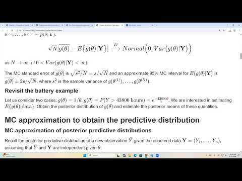
For N IID posterior draws, the average of g(θ) estimates E[g(θ) | data]; the Central Limit Theorem gives its approximate sampling distribution as N grows.
Estimate Monte Carlo standard error as the sample standard deviation of the g(θ) draws divided by √N.
An approximate 95% Monte Carlo interval is the estimate plus or minus about two Monte Carlo standard errors.
Sinha clarifies that N is the number of posterior draws, not the observed-data sample size.

6:20 Battery-Life Probability: Posterior Summaries and a 95% Credible Interval

For an exponential battery-life model, the chance a battery lasts beyond 43,800 hours is g(θ) = exp(−43,800θ).
Transform each posterior θ draw to obtain a sample from the posterior distribution of this probability, then summarize it with means, medians, and quantiles.
The estimated posterior mean is 0.312, median 0.303, and standard deviation 0.11; the 95% credible interval is approximately 0.12–0.558.
The Bayesian interval directly assigns 95% posterior probability to the interval given the observed data, unlike a frequentist confidence interval interpretation.

16:56 Posterior Predictive Distributions: Future Outcomes and Parameter Uncertainty

A posterior predictive distribution describes a future observation conditional on the data, integrating the likelihood over the posterior distribution of θ.
Sinha distinguishes a predictive interval for a future observation from a credible interval for an unknown parameter or parameter function.
A student asks whether these intervals are the same; Sinha explains that the ideas are related, but predictive intervals concern new observations.
For the battery example, the future lifetime distribution combines exponential sampling variability with uncertainty in θ.

20:48 Simulating Battery Lifetimes from the Posterior Predictive Distribution

For each iteration, draw θ from its posterior and then draw a future battery lifetime from an Exponential(θ) distribution.
Repeat the paired draws to approximate the full predictive distribution; R vectorization can perform the simulation more efficiently than an explicit for loop.
The simulated future battery-life distribution is broad, producing a much wider 95% predictive interval than an interval for a posterior mean.
For a continuous future outcome, inspect the simulated distribution or its histogram rather than focusing on a density value at one exact point.

29:23 Gamma–Poisson Conjugacy and Predictive Probabilities for Hospital Arrivals

For IID Poisson observations with mean θ and a Gamma(a,b) prior, the posterior is Gamma(a + nȳ, b + n), using the rate parameterization.
The exact posterior predictive distribution is negative binomial, but deriving it algebraically requires integration; Monte Carlo estimates it by averaging Poisson probabilities over posterior θ draws.
In the hospital example, 10 July days of emergency arrivals from 9–10 a.m. are modeled with a Poisson likelihood and a Gamma(1,1) prior.
The posterior predictive probability is estimated separately for counts such as 0, 1, and 2; the resulting probabilities can be displayed with a lollipop plot.

38:22 Posterior Predictive Checks Test the Poisson Assumption

Posterior predictive checking assesses whether data generated under the fitted model resemble the observed data; it remains necessary regardless of sample size.
Compare the empirical distribution with the posterior predictive distribution, or compare targeted summaries such as the mean, standard deviation, median, quartiles, and zero-count proportion.
A model is an approximation rather than a perfect account of reality, so the goal is to identify substantial mismatches rather than demand exact agreement.
For the hospital counts, Sinha compares observed summaries with summaries from the Poisson posterior predictive distribution.

42:35 Comparing Observed Counts with Predictive Summaries

The posterior predictive count distribution has mean about 3.91, median 4, and standard deviation about 2.06; the observed sample mean is 4.2 and standard deviation about 1.61.
The observed median is 4, matching the predictive median; observed quartiles are about 3.25 and 4.75, compared with predictive quartiles of 2 and 5.
No observed zero counts contrasts with a posterior predictive zero proportion of about 0.024, a plausible difference for a sample of only 10 days.
Sinha concludes that these summaries show no major mismatch, so the Poisson assumption appears reasonable, though not necessarily perfect.

47:20 Direct Predictive Simulation and the Next Lecture

An alternative to calculating predictive means and variances from a probability mass function is to draw one new Poisson observation for every posterior θ draw.
With many replicated observations—for example, 100,000—the sample directly approximates the posterior predictive distribution and supports ordinary summary calculations.
Sinha previews hierarchical models and sampling as the topic of the next class.

Summary, takeaways, and chapters were generated by AI from the video's transcript and may contain errors. The video belongs to its creator, Samiran Sinha.