STAT 638 (Fall 2026), Lecture 7

Overview

Samiran Sinha moves from a binomial survey example to Monte Carlo integration, showing how posterior calculations can be approximated with random draws when analytic integration is inconvenient. With 57 successes in 100 trials and a Beta(2,2) prior, he demonstrates estimating posterior means, variances, and probabilities, then applies the same approach to the mean lifetime of a phone battery.

Key takeaways

For 100 Bernoulli observations with 57 successes, inference about θ can use either the full Bernoulli likelihood or the binomial likelihood for the total; the binomial coefficient is constant in θ.
A uniform Beta(1,1) prior with 57 successes and 43 failures yields a Beta(58,44) posterior, while a Beta(2,2) prior yields Beta(59,45).
A Monte Carlo estimate of a posterior expectation is the average of g(θ) over posterior draws; increasing the number of draws generally reduces simulation variability.
For the Beta(59,45) posterior, the mean is about 0.5673 and the variance about 0.00233; 10,000 simulated draws closely approximate both quantities.
Posterior probabilities such as P(θ≤0.5) can be estimated by counting qualifying posterior draws; the example’s probability is about 0.083.
When θ is a gamma-distributed exponential rate, reciprocal draws 1/θ provide Monte Carlo samples of the corresponding battery mean lifetime without deriving its inverse-gamma summaries analytically.

Chapters

0:00 Project Checks and the 100-Person Policy Survey

Samiran Sinha asks students to begin their projects early and verify that datasets are accessible and research questions are reasonable.
The survey example samples 100 people from a much larger county population and records support for a policy as binary outcomes.

2:00 Bernoulli Likelihood and the Binomial Success Count

Each response Yᵢ is conditionally Bernoulli with success probability θ; the 100 observations are conditionally IID.
For a particular sequence with y successes, the likelihood is θʸ(1−θ)^(100−y); for the total Y=y, the binomial probability includes the coefficient choose(100,y).
The binomial coefficient does not depend on θ, so the individual-observation and success-count likelihoods give the same inference about θ.

4:54 Plotting the Likelihood for 57 Successes

With y=57 and n=100, Sinha evaluates the binomial probability across θ values from 0 to 1 in increments of 0.1.
The R demonstration uses the binomial probability mass function, dbinom, to calculate the probability of 57 successes for each candidate θ.
The plotted likelihood is largest near the observed success proportion, 57/100 = 0.57.

10:23 Discrete and Continuous Uniform Priors for θ

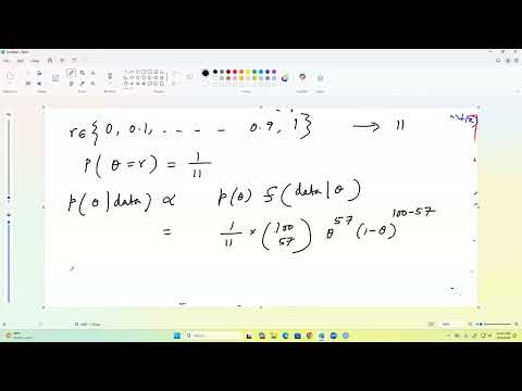
For a discrete uniform prior over 11 grid values, each θ value has prior probability 1/11; posterior probabilities are normalized likelihood values.
The discrete posterior plot contrasts the likelihood across θ with the updated posterior probabilities after observing 57 successes.
With a continuous uniform prior density on [0,1], the posterior is Beta(58,44), from adding 57 successes and 43 failures to the Beta(1,1) prior.
Sinha asks students to compare the discrete posterior, the continuous beta posterior density, and the uniform prior.

22:50 Project Coding Guidance and Exercise Practice

Students may use Python, but Sinha asks them to convert their code to R with tools such as ChatGPT or Claude so he can review it.
He recommends checking converted code by running it and verifying that it reproduces the original results.
Exercise 3.2 and related problems provide practice for numerical questions that may appear on quizzes and exams.

24:36 Monte Carlo Integration and the Law of Large Numbers

Monte Carlo methods approximate difficult integrals by averaging a large number of random samples.
The law of large numbers says the sample average of g(X) converges to its expectation when the expectation exists.
In Bayesian inference, draws θ₁,…,θₙ from the posterior let the average of g(θ) approximate its posterior expectation.
Posterior predictive distributions are one setting where integrating over the posterior parameter can be difficult.

30:17 Estimating Beta Posterior Means and Variances

For 57 successes and a Beta(2,2) prior, the posterior is Beta(59,45); 10,000 simulated draws produce a mean near 0.5672.
The analytical posterior mean is 59/(59+45), about 0.5673, illustrating the small sampling error in the Monte Carlo estimate.
The analytical posterior variance is about 0.00233, compared with a simulated estimate near 0.00236 from 10,000 draws.
Smaller draw counts, such as 100, produce more variable estimates because each result depends on random sampling.

38:09 Posterior Probabilities and the Empirical Distribution

The posterior probability P(θ≤0.5) can be estimated by the fraction of posterior draws at or below 0.5.
For the Beta(59,45) posterior, the theoretical probability is approximately 0.083; Monte Carlo estimates vary slightly around that value.
A histogram of 10,000 posterior draws approximates the beta density, so the empirical distribution also visualizes the posterior.

43:32 Phone Battery Lifetimes and Reciprocal Gamma Draws

In the exponential battery-lifetime example, the posterior for the rate θ is Gamma with shape 10 and rate 355940.
The mean battery lifetime is ψ=1/θ; because θ has a gamma distribution, ψ has an inverse-gamma distribution.
Sinha generates 10,000 gamma draws in R, takes their reciprocals, and averages them to estimate the posterior mean lifetime.
Repeated simulations give slightly different estimates—roughly 395 to 397 in the demonstration—while larger samples reduce Monte Carlo variability.

Summary, takeaways, and chapters were generated by AI from the video's transcript and may contain errors. The video belongs to its creator, Samiran Sinha.