STAT 638 (Fall 2026), Lecture 20

Overview

Samiran Sinha concludes the hierarchical-model discussion by interpreting hospital mortality estimates, MCMC diagnostics, and shrinkage, then introduces Bayesian linear regression. He shows how proposal scale affects Metropolis acceptance and autocorrelation, derives the frequentist least-squares/MLE estimates, and connects a normal prior for regression coefficients to their Bayesian full conditional distribution.

Key takeaways

Hierarchical pooling moves noisy hospital mortality estimates toward the overall pattern: Hospital A shifts from an observed rate near 20% to a posterior mean near 14%, while Hospital C shifts from about 9% toward 10%.
A high Metropolis acceptance rate is not by itself evidence of an efficient chain: reducing the proposal standard deviation to 0.2 raised acceptance to about 95% but increased autocorrelation and repeated-estimate variability.
For the normal regression model, maximizing the likelihood for β yields the ordinary least-squares estimator (XᵀX)⁻¹XᵀY.
With a diffuse normal prior on β, the Bayesian full conditional mean and covariance approach the frequentist estimate β̂ and its covariance sigma squared (XᵀX)⁻¹.
Endogeneity occurs when predictors are associated with regression errors; omitted variables can cause this problem in observational studies, even though the lecture assumes it away for the basic model.

Chapters

0:00 Hospital Mortality as a Hierarchical Model

The example estimates 30-day mortality probabilities for five hospitals using patient admission and death counts.
Hierarchical modeling lets hospitals with fewer admissions borrow information from hospitals in the same geographic region.
The model places distributions on hospital-specific probabilities and hyperparameters; Gibbs sampling is combined with Metropolis–Hastings for alpha and beta.

5:35 Diagnosing MCMC Convergence and Autocorrelation

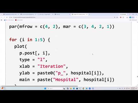
Trace plots for hospital probabilities P1–P5 and hyperparameters alpha and beta are used to assess whether chains have settled into stable bands.
The alpha and beta traces move closely from iteration to iteration, indicating high autocorrelation despite appearing to converge.
ACF plots show relatively little autocorrelation for hospital probabilities but substantial autocorrelation for alpha and beta.
With proposal standard deviations of 0.5, the Metropolis acceptance rates for alpha and beta are about 40% and 41%.

11:50 Mortality-Rate Shrinkage and Posterior Comparisons

Posterior means and 95% credible intervals are compared with raw hospital mortality rates; hierarchical estimates move toward the 45-degree equality line.
Hospital A’s observed mortality is about 20%, while its posterior mean is closer to 14%; Hospital C’s estimate moves from about 9% toward 10%.
The posterior probability that Hospital A’s mortality exceeds 15% is reported as 0.15.
The posterior probability that Hospital A’s mortality exceeds Hospital E’s is about 83%, supporting a probabilistic comparison rather than a raw-rate ranking.

17:03 Proposal Scale, Acceptance, and MCMC Efficiency

Sinha demonstrates random-walk Metropolis sampling from a known normal target with mean 1 and standard deviation 2, using 10,000 iterations and discarding 1,000 as burn-in.
Reducing the proposal standard deviation to 0.2 raises acceptance to about 95%, but produces highly autocorrelated draws and unstable run-to-run sample means such as 0.82, 0.92, and 1.03.
A larger proposal scale gives lower autocorrelation and repeated estimates near 1, including 1.003, 1.02, and 0.999.
Across repeated chains, both settings estimate the mean near 1, but the high-autocorrelation setting has much greater variability: about 0.21 versus 0.033.

28:32 Why Regression Relates Outcomes to Covariates

Regression studies associations between an outcome and variables called covariates, predictors, or control variables.
Sinha presents regression as a starting point for studying effects, while noting that causal inference is a separate topic.
The course proceeds from linear regression to generalized linear models, where outcomes may follow distributions such as Poisson rather than normal.

31:39 Linear Regression in Vector and Matrix Form

Linear regression uses a numeric outcome Y and predictors X1 through XP, with coefficients beta1 through betaP and an error term.
The model is written as Y = Xᵀβ + ε for an observation, or as bold Y = Xβ + ε across N observations.
For N observations and P predictors, the response and error are N×1 vectors, the design matrix is N×P, and β contains the unknown regression coefficients.
The error is modeled as mean-zero normal noise with variance sigma squared, representing variation not captured by the predictors.

36:38 Regression Assumptions and Endogeneity

The observed response Y and design matrix X are treated as known, while β, sigma squared, and the latent errors are unknown.
A central condition is that the conditional mean of the error given X is zero; the standard model also assumes independent normal errors with covariance sigma squared times the identity matrix.
Dependence between predictors and errors creates endogeneity, which can arise from omitted variables in observational studies in fields such as economics and sociology.
Sinha assumes no endogeneity for the course’s regression treatment and contrasts controlled experiments with data collected from nature.

39:20 Frequentist Linear Regression: Least Squares and MLE

Under independent normal errors, the likelihood for β and sigma squared is based on the residual vector Y − Xβ.
Maximizing the likelihood for β is equivalent to minimizing the residual sum of squares, giving β̂ = (XᵀX)⁻¹XᵀY.
The MLE for sigma squared is the residual sum of squares divided by N; the hat matrix H is symmetric and idempotent.
The least-squares estimate of β also applies under weaker assumptions of zero conditional error mean and finite conditional variance.

43:17 Bayesian Regression Priors and Posterior Construction

The Bayesian model combines the regression likelihood with a multivariate normal prior for the coefficient vector β.
A prior mean β₀ and prior covariance matrix are specified for β; sigma squared receives an inverse-gamma prior, as in normal-model inference from Chapter 5.
The joint posterior for β and sigma squared is proportional to the likelihood multiplied by both parameter priors.
Introducing predictors replaces the simple normal-model mean μ from Chapter 5 with Xᵀβ.

47:01 The Beta Full Conditional and Its Link to MLE

Completing the square in the posterior gives a normal full conditional distribution for β given sigma squared and the data.
As the prior precision approaches zero, corresponding to a very diffuse prior, the conditional mean becomes the least-squares estimate β̂.
In the same diffuse-prior limit, the conditional covariance becomes sigma squared times (XᵀX)⁻¹, matching the frequentist sampling covariance of β̂.
The Bayesian distribution describes the unknown β given fixed data, whereas the frequentist distribution describes β̂ as a random function of data with fixed unknown β.

Summary, takeaways, and chapters were generated by AI from the video's transcript and may contain errors. The video belongs to its creator, Samiran Sinha.