STAT 638 (Fall 2026), Lecture 15

Overview

Samiran Sinha reviews Bayesian quiz problems on Poisson and binomial data, conjugate beta updates, mixture priors, posterior uncertainty, and posterior prediction. He then begins Homework 6, Exercise 6.3, introducing a probit model for divorce outcomes and deriving the structure of the full conditional for its regression coefficient.

Key takeaways

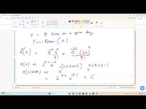
Independent Poisson counts add their rates: 4 cases on one day and 9 cases across two days, under a Gamma(2, 1) prior, produce a Gamma(15, rate 4) posterior and an approximate 95% interval of 2.10–5.87.
A Beta(3, 3) prior updated with 9 successes and 3 failures gives Beta(12, 6); posterior odds above 0.8 require dividing the upper-tail probability by its complementary probability, not reporting the tail probability alone.
A mixture prior’s posterior component weights are not generally unchanged: the Beta(1, 1) and Beta(10, 3) components update to Beta(18, 9) and Beta(27, 11), with weights adjusted by their marginal likelihoods.
Monte Carlo can estimate mixture uncertainty and predictive probabilities directly: Sinha’s 60,000/40,000 mixture draws gave a standard deviation near 0.282 and an estimated probability near 0.239 of exactly 4 survivals in 5 future plants.
In the probit model Zᵢ = βXᵢ + εᵢ with standard normal errors, conditioning on latent Z makes the normal-prior full conditional for β Gaussian and removes any additional β-dependent contribution from observed Y.

Chapters

0:00 Using AI Without Losing STAT 638 Learning Objectives

Samiran Sinha encourages AI use for class notes and projects but warns against relying on it blindly.
Quizzes and exams are open book, open note, and open internet; Sinha emphasizes applying methods to real problems rather than prioritizing grades.
Sinha says future quizzes will allow 20 minutes instead of 15, responding to student feedback.

2:30 Poisson Admissions Data: Gamma Posterior and 95% Interval

The example observes 4 admissions on day 1 and 9 admissions across days 2 and 3; the latter total follows Poisson with rate 2λ.
With independent observations and a Gamma(2, 1) prior, the posterior for λ is Gamma(15, rate 4).
Using R to obtain the 2.5th and 97.5th percentiles gives an approximate 95% credible interval of 2.10 to 5.87.

8:35 Distinguishing Posterior Odds from Probability

For 9 successful jobs in 12 attempts, the binomial likelihood is proportional to θ⁹(1−θ)³; the factor 12 choose 9 cancels in posterior calculations.
Sinha distinguishes odds from probability: odds for an event equal its probability divided by the probability of its complement.
The prior is Beta(3, 3), and the observed successes and failures update the model.

11:55 Beta(12, 6) Posterior Odds Above an 0.8 Success Rate

Combining the Beta(3, 3) prior with 9 successes and 3 failures yields a Beta(12, 6) posterior for θ.
The requested posterior odds are P(θ > 0.8 | data) divided by P(θ ≤ 0.8 | data), computed from beta-distribution integrals.
When rewriting the lower-tail probability as one minus the upper-tail probability, the common Beta(12, 6) normalizing constant must be handled consistently.

18:30 Updating a Two-Component Beta Mixture for Plant Survival

Of 25 tracked plants, 17 survive; the prior assigns equal weight to Beta(1, 1) and Beta(10, 3).
The binomial likelihood updates the components to Beta(18, 9) and Beta(27, 11), respectively.
The posterior remains a two-component beta mixture, but its weights change according to each component’s marginal likelihood; mixture normalization constants cannot be discarded.

31:50 Monte Carlo Standard Deviation for a Beta Mixture

For a posterior with 60% weight on Beta(1, 1) and 40% on Beta(15, 3), Sinha estimates the standard deviation by sampling from each component.
He combines 60,000 uniform draws from Beta(1, 1) with 40,000 draws from Beta(15, 3), then calculates the sample standard deviation.
Monte Carlo estimates vary slightly across runs, with examples near 0.282; the answer choices identify approximately 0.282.

34:48 Predicting Four Survivors Among the Next Five Plants

The target is the posterior predictive probability that exactly 4 of the next 5 plants survive under the same 60% Beta(1, 1) and 40% Beta(15, 3) mixture.
For each posterior draw θ, Sinha evaluates the binomial probability 5 choose 4 times θ⁴(1−θ), then averages those probabilities.
Using posterior draws from the preceding Monte Carlo calculation gives an estimate near 0.239, with small run-to-run variation.

41:38 Homework 6 Access and the Divorce Panel-Study Exercise

Sinha explains that some notation disappeared in the accessible copy of the book exercises and directs students to a Google Drive link.
Students need a TAMU NetID and password to access the exercise document; the link is provided because the source document cannot simply be posted in an inaccessible format.
Exercise 6.3 concerns a five-year panel study of 25 married couples and uses the file divorce.dat.

45:43 Probit Model for Divorce and Spouses’ Age Difference

The response Yᵢ records a binary divorce outcome, while Xᵢ is the husband’s age minus the wife’s age.
The latent-variable model is Zᵢ = βXᵢ + εᵢ, with independent standard normal errors; Yᵢ is 1 when Zᵢ exceeds threshold C and 0 otherwise.
The sign of β indicates how age difference relates to divorce probability: positive β raises the probability as Xᵢ increases, while negative β lowers it.

48:18 Gaussian Full Conditional for the Probit Regression Coefficient

For the conditional distribution of β given Y, X, Z, and C, Sinha combines the latent-variable likelihood Zᵢ | β ~ Normal(Xᵢβ, 1) with a normal prior for β.
Because the likelihood and prior are Gaussian, the full conditional for β is also normal, with its mean and variance obtained by combining their precision contributions.
Once Z is conditioned on, Y contributes no additional β-dependent factor; the lecture ends after starting this part of Exercise 6.3.

Summary, takeaways, and chapters were generated by AI from the video's transcript and may contain errors. The video belongs to its creator, Samiran Sinha.