STAT 638 (Fall 2026), Lecture 12

Overview

Samiran Sinha develops Bayesian inference for a normal model with unknown mean and variance, using precision θ₂ = 1/σ² and a conjugate normal-gamma prior to derive the posterior. He then derives the Jeffreys-prior posterior and demonstrates posterior sampling in R on ball-bearing measurements, including credible intervals, HPD intervals, and inference for functions of the parameters.

Key takeaways

With θ₂ defined as precision, the normal-gamma prior uses θ₁ | θ₂ ~ Normal(μ₀, 1/(κ₀θ₂)) and θ₂ ~ Gamma(A₀, B₀), yielding a conjugate posterior.
Under the Jeffreys prior proportional to θ₂⁻¹ᐟ², the normal-model posterior has θ₁ | θ₂, Y ~ Normal(ȳ, 1/(nθ₂)) and θ₂ | Y ~ Gamma(n/2, (n−1)s²/2) in shape-rate form.
The ball-bearing example’s sample mean of about 2.4918 closely matches its posterior mean of about 2.491865; its 95% credible interval for the population mean is about 2.4879–2.4957.
Transforming precision draws with σ² = 1/θ₂ produces a skewed variance posterior, for which equal-tail and HPD intervals may differ substantially.
A joint posterior sample supports inference for derived quantities such as the coefficient of variation, √(1/θ₂)/θ₁, by transforming each paired draw.

Chapters

0:00 Normal Inference with Unknown Mean and Precision

The model treats Y₁,…,Yₙ as normal observations with unknown mean θ₁ and precision θ₂ = 1/σ².
The parameter space is θ₁ ∈ ℝ and θ₂ > 0; inference concerns population parameters, not just the observed sample mean and variance.
Sinha frames the normal model as a foundation for methods that can extend to more complex statistical problems.

5:00 A Conjugate Normal-Gamma Prior and Its Marginals

The prior specifies θ₁ | θ₂ as Normal(μ₀, 1/(κ₀θ₂)) and θ₂ as Gamma(A₀, B₀), with Gamma expressed using a rate parameter.
The values μ₀, κ₀, A₀, and B₀ are hyperparameters; fixing them gives the normal-gamma prior its conjugate structure.
Although θ₂ has a gamma marginal, integrating it out makes θ₁ marginally a nonstandardized t-distribution rather than a normal distribution.
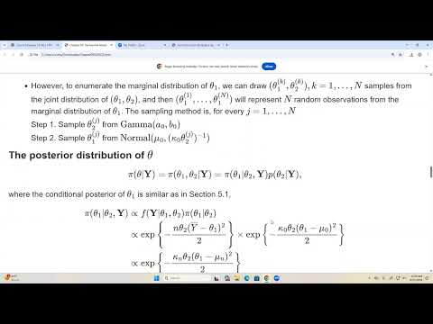
To simulate from the joint prior, first draw θ₂, then draw θ₁ conditional on that θ₂; repeated draws also reveal marginal distributions.

10:00 Deriving the Normal-Gamma Posterior

The joint posterior factors into θ₁ | θ₂, Y and θ₂ | Y, separating a conditional posterior from a marginal posterior.
Completing the square in θ₁ gives a normal conditional posterior with κₙ = κ₀ + n and mean μₙ = (κ₀μ₀ + nȳ)/κₙ.
Integrating θ₁ out uses the normal-sum identity: with the normal-gamma prior, each Yᵢ marginally given θ₂ is normal with mean μ₀ and variance 1/θ₂ + 1/(κ₀θ₂).
The resulting posterior remains normal-gamma: θ₂ | Y is gamma, and θ₁ | θ₂, Y is normal, enabling direct posterior summaries.

16:00 Posterior Means and Credible Intervals from Draws

Posterior means can be estimated by averaging sampled θ₁ or θ₂ values from the joint posterior.
A 95% equal-tail credible interval uses the 2.5th and 97.5th percentiles of the relevant posterior draws.
The same posterior sample supports summaries for both parameters without separately deriving every requested statistic.

23:00 Jeffreys Prior for the Normal Mean and Precision

For one normal observation with mean θ₁ and precision θ₂, the Fisher information matrix has diagonal entries θ₂ and 1/(2θ₂²), with zero cross-information.
The determinant is 1/(2θ₂), so Jeffreys prior is proportional to θ₂⁻¹ᐟ².
Under this prior, the posterior conditional for θ₁ is normal with mean ȳ and variance 1/(nθ₂).
The marginal posterior for θ₂ is Gamma with shape n/2 and rate (n−1)s²/2, where s² is the sample variance.

28:00 Ball-Bearing Data and Translating Formulas into R

Sinha applies the Jeffreys-prior method to ball-bearing measurements, targeting the population mean and variance through θ₁ and θ₂.
He distinguishes the sample average from the unknown population mean and the sample variance from the population variance.
Sinha argues that understanding the formulas is necessary to check and guide code generated with tools such as Claude or ChatGPT.
The implementation uses the sample size n, sample mean ȳ, and sample variance s² to parameterize posterior draws.

33:00 Sampling Joint Posterior Draws in R

The R procedure draws θ₂ from a gamma distribution with shape n/2 and rate (n−1)s²/2.
For each θ₂ draw, it samples θ₁ from Normal(ȳ, 1/(nθ₂)); this conditional step must be repeated inside the loop.
A loop of 10,000 iterations stores θ₁ and θ₂ in a two-column matrix for subsequent summaries.
Sinha checks the scale and parameterization before running the loop, emphasizing that a gamma rate multiplies θ₂ in the exponential while a scale is its reciprocal.

37:00 Ball-Bearing Mean: Posterior Estimates and Probability

The observed sample mean is approximately 2.4918, while the posterior mean of θ₁ is approximately 2.491865.
The 95% equal-tail credible interval for θ₁ is approximately 2.4879 to 2.4957.
The posterior probability that θ₁ exceeds 2.50 is estimated from the draws at roughly 0.0002.
Increasing the number of Monte Carlo draws can improve the precision of estimated posterior probabilities and quantiles.

42:00 Variance Posterior, Skewness, and HPD Intervals

Variance draws are obtained by transforming each precision draw as σ² = 1/θ₂; the resulting posterior distribution is skewed.
The variance posterior median is approximately 3.97 × 10⁻⁵, with a 95% equal-tail interval of roughly 1.939 × 10⁻⁵ to 1.019 × 10⁻⁴.
Sinha introduces highest posterior density intervals (HPDIs) as an alternative to percentile-based credible intervals and demonstrates calculating them from posterior samples.
Equal-tail and HPD intervals can differ noticeably for skewed distributions, while they tend to be closer for approximately symmetric distributions.

48:00 Using Joint Draws for the Coefficient of Variation

Posterior draws for any function of the parameters can be computed by transforming each paired draw from the joint posterior.
For the coefficient of variation σ/μ, each draw can be transformed as √(1/θ₂)/θ₁.
The transformed draws provide posterior means, credible intervals, and probability calculations for derived quantities without a separate analytic posterior derivation.

Summary, takeaways, and chapters were generated by AI from the video's transcript and may contain errors. The video belongs to its creator, Samiran Sinha.