STAT 638 (Fall 2026), Lecture 5

Overview

Samiran Sinha develops Bayesian inference for Poisson counts, moving from the likelihood and maximum-likelihood estimate to Gamma conjugate priors, Jeffreys priors, and mixture priors. Using plastic-film blemish counts, including observations collected over varying areas, he derives posterior distributions, discusses prior sensitivity and sample-size planning, and demonstrates a two-component Gamma mixture with a posterior mean of 0.2932.

Key takeaways

For n IID Poisson counts, the sufficient statistic is the total count ∑Yᵢ, and the maximum-likelihood rate estimate is the sample mean.
A Gamma(A, B) prior for a Poisson rate yields a Gamma(A + ∑Yᵢ, B + n) posterior when B is parameterized as a rate.
Jeffreys prior for a Poisson rate is proportional to θ^(−1/2); although improper on (0, ∞), it gives a proper posterior after at least one observation.
When counts are collected over different areas Wᵢ, the correct rate estimate is total counts divided by total area, ∑Yᵢ/∑Wᵢ.
A mixture prior updates component by component, and each posterior mixture weight is proportional to the prior weight times that component’s marginal likelihood.
Prior sensitivity has no fixed sample-size cutoff; compare plausible priors for existing data, or plan a Bayesian study around a target posterior probability before collecting data.

Chapters

0:00 Poisson Blemish Counts and the Role of Sampling Design

Sinha follows the binomial-inference structure—likelihood, prior choice, and posterior inference—for the Poisson model.
For a random sample of independent observations, the joint distribution is the product of individual probability mass functions.
The likelihood must reflect the sampling design; changing how observations are collected can change the likelihood and invalidate inference if ignored.
For a homogeneous Poisson process, expanding the observed area scales the mean by the area, such as multiplying the per-square-centimeter rate by 11.

5:00 Poisson Likelihood, Sufficient Statistic, and Maximum-Likelihood Estimate

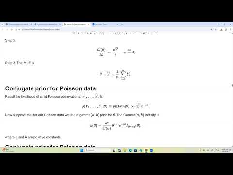
For n IID Poisson observations with rate θ, the likelihood is proportional to θ^(nȳ)e^(-nθ).
The sum of counts, equivalently nȳ, is sufficient for θ, so inference does not require retaining each observation separately.
Taking the log likelihood and setting its derivative to zero gives the MLE θ̂ = ȳ.
A second derivative evaluated at the estimate can verify that the log likelihood is maximized.

8:35 Gamma Conjugacy for the Poisson Rate

A Gamma prior with shape A and rate B has kernel θ^(A−1)e^(−Bθ), matching the Poisson likelihood’s dependence on θ.
Multiplying the prior and likelihood gives a Gamma posterior with shape A + nȳ and rate B + n.
Conjugacy makes posterior summaries such as means and standard deviations straightforward to calculate.
Sinha notes that conjugacy is convenient rather than mandatory; modern computation also permits nonconjugate priors.

12:50 Jeffreys Prior: Fisher Information and Posterior Properness

For one Poisson observation, the expected Fisher information is 1/θ, giving Jeffreys prior π(θ) ∝ θ^(−1/2).
The prior is improper because integrating θ^(−1/2) over 0 to ∞ diverges.
Combining it with n IID Poisson observations produces a Gamma posterior with shape 1/2 + nȳ and rate n.
That posterior is proper for n ≥ 1, illustrating why an improper prior can still be usable when the resulting posterior is proper.

20:00 Jeffreys Prior for IID Data and Area Offsets

For IID observations, Fisher information from n observations is n times the information from one observation; the factor n vanishes in the proportionality constant of Jeffreys prior.
Sinha recommends deriving Jeffreys prior from one observation to reduce calculation errors, while limiting the equivalence claim to the IID setting.
With sampled area ω, a blemish count has Poisson mean ωθ and the information is ω/θ.
Because ω is known, its factor is absorbed into the proportionality constant, leaving π(θ) ∝ θ^(−1/2).

28:00 Mixture Priors: Weighted Densities, Not Weighted Random Variables

A mixture prior is a weighted sum of proper densities, with nonnegative weights summing to 1; the resulting prior is proper.
Sinha illustrates a 10:8 mixture of Normal(0, 1) and Normal(3, 0.25), which produces a visibly bimodal density in the example.
A mixture of densities is not the same as a weighted average of two random variables: the latter is normally distributed when its components are independent normals.
After observing data, the posterior remains a mixture, with updated component densities and weights.

34:30 Varying Observation Areas: Poisson Likelihood and Rate Estimate

For observation i, the blemish count Yᵢ is modeled as Poisson with mean Wᵢθ, where Wᵢ is the sampled area.
The likelihood accounts for differing areas through the exposure term involving θ∑Wᵢ.
Setting the score function to zero yields θ̂ = ∑Yᵢ / ∑Wᵢ: total blemishes divided by total observed area.
The example’s frequentist estimate is 0.2910 blemishes per square centimeter.

37:20 Posterior Comparisons, Prior Sensitivity, and Study Design

With a Gamma(A, B) prior, the varying-area posterior has shape A + ∑Yᵢ and rate B + ∑Wᵢ; Jeffreys prior uses A = 0.5 and B = 0.
Posterior curves under several Gamma hyperparameter choices remain concentrated roughly between 0.2 and 0.4 in this dataset.
There is no universal sample-size threshold for prior sensitivity; analysts should compare posteriors across plausible hyperparameters.
Before data collection, Bayesian trial design can choose a sample size to target a posterior probability, such as an 80% probability that a drug success rate exceeds a specified value.

44:30 Two-Component Gamma Mixture: Posterior Components and Weights

Sinha constructs a prior from two Gamma distributions, with parameters (A₁, B₁) and (A₂, B₂) and weights K₁ and K₂ summing to 1.
Each prior component updates to its own Gamma posterior, while the overall posterior remains a two-component mixture.
The updated weight for component j is proportional to its prior weight Kⱼ times its marginal-likelihood constant Cⱼ, then normalized across components.
Writing the normalizing constants explicitly is essential for obtaining the posterior mixture weights.

48:35 Numerical Gamma Mixture: Stable Computation and Posterior Summaries

The numerical illustration mixes Gamma(1, 10) and Gamma(2, 2) priors with weights 0.1 and 0.9.
Very small likelihood terms can cause numerical 0/0 or NaN results; computing on the log scale helps avoid underflow.
Simulating from the resulting posterior mixture places most probability between 0.25 and 0.35 blemishes per square centimeter.
The mixture posterior mean is 0.2932; simulation also supplies empirical estimates of the median and standard deviation.

Summary, takeaways, and chapters were generated by AI from the video's transcript and may contain errors. The video belongs to its creator, Samiran Sinha.