STAT 638 (Fall 2026), Lecture 13

Overview

Samiran Sinha finishes the normal-model material in Chapter 5 by using posterior simulation to summarize the coefficient of variation and approximate the posterior predictive distribution for future observations. He then introduces Gibbs sampling for complex Bayesian posteriors, derives the full conditional distributions for a normal model with conjugate priors, and explains initialization, dependence, burn-in, and trace-plot checks before setting up a propellant-burning-rate example.

Key takeaways

The posterior predictive distribution for a future normal observation is a mixture over posterior uncertainty in both the mean theta1 and precision theta2; Monte Carlo draws provide a practical approximation when the integral is hard to evaluate.
In R's rnorm function, the third argument is the standard deviation, so the normal-model input must be sqrt(1/theta2), not the variance 1/theta2.
Gibbs sampling updates one parameter at a time from its full conditional, using the latest available values of the other parameters.
For the conjugate normal model, theta1 given theta2 and the data is normal with mean (n*ybar + kappa0*mu0)/(n+kappa0) and variance 1/((n+kappa0)*theta2).
Gibbs draws are dependent across iterations; burn-in and trace plots help assess whether the chain has moved away from its initial values and is sampling from the target posterior.
Initial values can materially affect difficult, high-dimensional computations: Sinha reports using Lasso-based starts in a project with roughly 5,000 parameters rather than relying on random standard-normal starts.

Chapters

0:00 Lecture Plan and Quiz 2 Scope

Samiran Sinha plans to finish Chapter 5's normal-distribution example and begin Chapter 6 on Gibbs sampling.
The Friday class will not meet on campus; a recorded lecture will be available that day.
Quiz 2 covers Chapters 1–4, including model selection, but excludes the normal-distribution material.

3:00 Ball-Bearing Example: Coefficient of Variation

Sinha revisits Bayesian inference for the ball-bearing data under a Jeffreys prior.
For a normal model with variance 1/theta2, the standard deviation is 1/sqrt(theta2); the coefficient of variation is standard deviation divided by mean.
Posterior draws can be used to summarize the coefficient of variation and calculate quantiles.

6:00 Posterior Predictive Density as a Posterior Mixture

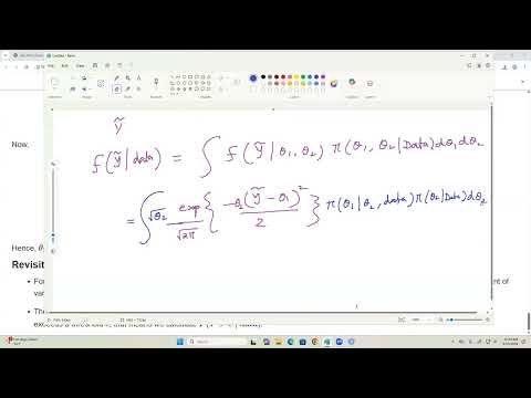
The predictive density for a future observation Y-tilde integrates its normal density over the posterior distribution of theta1 and theta2.
For fixed parameters, Y-tilde is normal with mean theta1 and standard deviation sqrt(1/theta2).
Sinha notes that evaluating the mixture density analytically is difficult, motivating Monte Carlo simulation.

9:30 Simulating Future Observations in R

Sinha reuses posterior draws stored in a matrix, with theta1 in column one and theta2 in column two.
For each posterior parameter draw, R's rnorm function generates a future observation using mean theta1 and standard deviation sqrt(1/theta2).
He emphasizes that rnorm expects a standard deviation, not a variance—a distinction that varies across software functions.

14:00 Prediction Intervals and Extreme-Event Probabilities

The simulated predictive distribution has an estimated mean of about 2.4918.
Sinha reports a 95% prediction interval of approximately 2.4778 to 2.505 for a future observation.
Monte Carlo draws estimate probabilities of threshold events, such as a future observation falling below 2.47; the reported estimate is 0.00218.
A histogram displays the predictive distribution, and kernel smoothing can replace its block-like appearance with a smooth curve.

16:30 Why Complex Bayesian Models Need Gibbs Sampling

Conjugate examples such as a binomial likelihood with a beta prior have easy-to-sample posterior distributions, but practical models often lack standard-form posteriors.
Posterior means, standard deviations, and credible intervals can be estimated by drawing numerical samples from the posterior.
Gibbs sampling extends the two-step normal-model sampling from Chapter 5 to settings where marginal posterior calculations are difficult.
Sinha cites the negative-binomial model, previously sampled using the BRMS package, as an example of more complex computation.

21:00 Gibbs Updates and Choosing Initial Values

For a parameter vector with M components, Gibbs sampling repeatedly draws each component from its full conditional distribution.
Each update conditions on the data and the most recently updated values of the other parameters.
Initial values are chosen by the practitioner; poor starting points can slow convergence or cause problems in high-dimensional models.
Sinha describes a project with about 5,000 parameters where Lasso-based initial values worked better than random draws from a standard normal distribution; prior draws are another option but may be poor with diffuse priors.

27:20 Normal-Model Full Conditional for the Mean

The model assumes IID normal observations with mean theta1 and variance 1/theta2, with theta1 conditional on theta2 normally distributed and theta2 given a gamma prior.
The full conditional for theta1 is obtained by retaining theta1-dependent terms in the joint posterior and completing the square.
The resulting conditional distribution is normal with mean (n times the sample mean plus kappa0 times mu0) divided by (n plus kappa0).
Its conditional variance is 1 divided by ((n plus kappa0) times theta2), so the variance changes with the current theta2 draw.

39:00 Gamma Update, Chain Dependence, and Burn-In

Collecting theta2-dependent terms in the joint posterior gives a gamma full conditional with shape a0 + (n+1)/2 and a rate that depends on theta1.
Unlike Chapter 5's marginal posterior for theta2, this conditional gamma distribution depends on the current theta1 and has different shape and rate parameters.
The alternating updates create dependent Markov-chain draws; Gibbs samples across iterations are not independent.
Early draws can reflect the initial values, so practitioners discard burn-in and inspect trace plots; the appropriate burn-in length depends on the model and chain behavior.

48:20 Propellant Example and Gibbs-Code Setup

Sinha introduces an engineering-statistics example about solid-propellant rocket systems, where the specified mean burning rate is 50 centimeters per second.
The example uses a sample of 25 observations and initializes theta1, the mean, at 0 and theta2, the precision, at 10.
Because the sample average is far from the initial theta1 value, the setup illustrates how a deliberately poor starting point affects the chain.
The lecture ends as Sinha begins coding the normal and gamma updates; he reserves the code output and interpretation for the next lecture.

Summary, takeaways, and chapters were generated by AI from the video's transcript and may contain errors. The video belongs to its creator, Samiran Sinha.