STAT 638 (Fall 2026), Lecture 3

Overview

Samiran Sinha develops Bayesian inference for binomial data from the Bernoulli trial model, showing how independent outcomes yield a likelihood determined by the total success count and how a Beta prior produces a Beta posterior. He works through a campus COVID-19 example with a Beta(2,20) prior and 25 cases among 100 students, obtaining a Beta(27,95) posterior and about a 70% probability that prevalence exceeds 20%, then derives the Beta conjugate update for a geometric likelihood.

Key takeaways

For n independent Bernoulli(theta) trials, the success count has mean n theta and variance n theta(1-theta), because the covariance terms vanish under independence.
The likelihood from individual Bernoulli responses depends on the data through T=sum Y_i; an aggregate count can therefore support inference about theta without exposing individual responses.
With a Beta(A,B) prior and Y successes in n binomial trials, the posterior is Beta(A+Y,B+n-Y), since the prior and likelihood exponents add.
In the campus example, Beta(2,20) combined with 25 cases among 100 students produces Beta(27,95) and an approximately 70% posterior probability that prevalence is greater than 20%.
For a geometric likelihood theta(1-theta)^(Y-1), a Beta(A,B) prior yields Beta(A+1,B+Y-1), demonstrating that conjugate families can be found by matching algebraic forms.

Chapters

0:00 Project Assignment Logistics and a Write-to-Learn Study Practice

Samiran Sinha asks students who have not yet added their names to the discussion board to do so before projects are randomly assigned.
The posted projects are intended to be non-textbook problems with potential to develop into publishable work.
Sinha recommends rewriting lecture derivations by hand as practice for solving unfamiliar problems.

2:19 Glossophobia Example: From One Bernoulli Trial to 30-Student Binomial Counts

A Bernoulli variable records whether one student has glossophobia: 1 for yes and 0 for no, with success probability theta.
Counting affected students among 30 independent students with a common probability theta gives a Binomial(30, theta) random variable.
The binomial model requires independent trials with the same success probability.

3:57 Bernoulli Mean and Variance Build the Binomial Moments

For a Bernoulli(theta) variable, the probability mass function is theta^y(1-theta)^(1-y) for y in {0,1}.
The Bernoulli mean is E(Y_i)=theta and its variance is Var(Y_i)=theta(1-theta).
Writing the count as Y=sum of n independent Bernoulli variables gives E(Y)=n theta and Var(Y)=n theta(1-theta); independence removes covariance terms.

8:29 IID Bernoulli Likelihood Depends on the Total Number of Successes

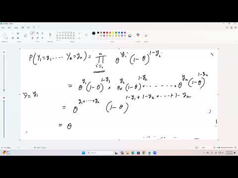
For independent observations Y_1,...,Y_n, multiplying their Bernoulli mass functions gives theta^T(1-theta)^(n-T), where T=sum Y_i.
The same likelihood can be expressed using the sample mean as theta^(n times the sample mean) times (1-theta)^(n minus n times the sample mean).
For inference about theta, the individual 0/1 responses enter the likelihood only through the total T.

16:01 Binomial Likelihood, Counting Combinations, and Privacy-Preserving Totals

When only the total Y is observed, its binomial likelihood includes the factor choose(n,Y) multiplying theta^Y(1-theta)^(n-Y).
The choose(n,Y) factor counts the possible arrangements of Y successes among n trials and is constant with respect to theta.
An experimenter can estimate prevalence from an aggregate count, such as the number of affected students out of 30, without receiving student-level responses.

20:10 Bayes' Rule: Posterior Proportional to Prior Times Likelihood

For Bernoulli observations, the posterior density is the prior density times theta^T(1-theta)^(n-T), divided by the marginal likelihood.
The marginal likelihood integrates over theta from 0 to 1 and is constant with respect to theta after integration.
Using the binomial likelihood gives the same posterior because choose(n,Y) appears in both numerator and denominator and cancels.
A proportional posterior can be normalized into a probability density by dividing by its integral.

27:05 Beta Priors Encode Beliefs About a Success Probability

A Beta(A,B) density on 0<theta<1 is proportional to theta^(A-1)(1-theta)^(B-1), with A>0 and B>0.
The normalizing constant is 1/B(A,B), where B(A,B)=Gamma(A)Gamma(B)/Gamma(A+B); the Beta distribution is distinct from the Beta function.
Beta(1,1) is uniform, Beta(0.5,0.5) puts more density near 0 and 1, and Beta(1,10) favors smaller success probabilities.
Changing A and B lets an analyst represent different prior beliefs about theta's likely values.

35:25 Campus COVID-19 Example: Beta(2,20) Updates to Beta(27,95)

Sinha uses a Beta(2,20) prior for campus COVID-19 prevalence, with prior mean 2/22, about 0.091, and standard deviation about 0.06.
Observing 25 infected students among 100 yields a Beta(2+25, 20+100-25)=Beta(27,95) posterior.
The posterior probability that prevalence exceeds 20% is the integral of the Beta(27,95) density from 0.2 to 1, calculated as 1 minus the Beta CDF at 0.2.
The example gives a posterior probability of roughly 70% that prevalence is above 20%.

43:35 Conjugate Priors: Beta Updates for Binomial and Geometric Data

A prior is conjugate when its posterior belongs to the same distribution family; Beta priors are conjugate for binomial likelihoods, with posterior Beta(A+Y,B+n-Y).
For a geometric likelihood proportional to theta(1-theta)^(Y-1), multiplying by a Beta(A,B) prior gives a Beta(A+1,B+Y-1) posterior.
The geometric update illustrates how to identify conjugacy by matching powers of theta and 1-theta in the likelihood-prior product.
Sinha assigns practice with these basic updates as preparation for Bayesian point estimation in the next class.

Summary, takeaways, and chapters were generated by AI from the video's transcript and may contain errors. The video belongs to its creator, Samiran Sinha.