Riemann sums (Calc 1; Lecture 3-6; Fall 26)
Overview
The lecture reviews polynomial long division and antiderivative strategies, then develops Riemann sums as rectangle-based estimates of area. Examples show left, right, and midpoint estimates for y = 4x² on [0,4] as 56, 120, and 84, apply a midpoint sum to tabulated data for an estimate of 22, and introduce sigma notation and the limit as the number of rectangles approaches infinity.
Key takeaways
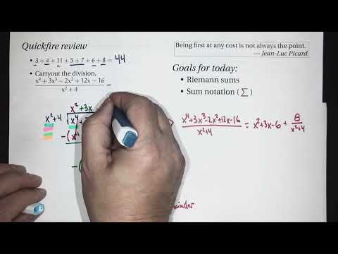
- Polynomial long division can be organized by repeatedly canceling leading terms; dividing x⁴ + 3x³ − 2x² + 12x − 16 by x² + 4 gives quotient x² + 3x − 6 and remainder 8.
- The integral ∫1/(x² + 4) dx becomes ½ arctan(x/2) + C after factoring out 4 and applying the chain-rule scaling correction.
- Multiplying 1/(1 + sin θ) by (1 − sin θ)/(1 − sin θ) converts it into sec²θ − sec θ tan θ, yielding tan θ − sec θ + C.
- For the increasing function 4x² on [0,4], four left rectangles estimate 56 and four right rectangles estimate 120; the four-midpoint estimate is 84.
- A midpoint sum can work from table values alone: three width-2 intervals on [1,7], with transformed inputs 7, 4, and 1, produce an estimate of 22.
- Sigma notation expresses repeated rectangle areas as Σ f(xₖ)Δx, and taking n to infinity with Δx = (b − a)/n leads to the limiting area calculation.
Chapters
- Divide x⁴ + 3x³ − 2x² + 12x − 16 by x² + 4 using leading terms to build the quotient.
- The quotient is x² + 3x − 6, and the remainder is 8, so the result is x² + 3x − 6 + 8/(x² + 4).
- At each step, multiply the divisor by the next quotient term, subtract, and stop when the remaining polynomial has degree below 2.
- For ∫1/(x² + 4) dx, do not split the denominator across addition; instead, factor out 4 to expose the form 1 + (x/2)².
- Use ∫1/(1 + x²) dx = arctan(x) + C and the chain-rule scaling correction to obtain ½ arctan(x/2) + C.
- Derivative review confirms the chain rule for sin(3x), cos(4x), and sec(5x), producing factors of 3, 4, and 5.
- To integrate 1/(1 + sin θ), multiply numerator and denominator by 1 − sin θ.
- Apply 1 − sin²θ = cos²θ to rewrite the integrand as (1 − sin θ)/cos²θ.
- Split the expression into sec²θ − sec θ tan θ, whose antiderivative is tan θ − sec θ + C.
- Riemann sums estimate the area under a curve by dividing an interval into strips and treating each strip as a rectangle.
- Each rectangle contributes height times width, with the height found by evaluating the function at a chosen point in its interval.
- Using more rectangles generally improves the approximation, but requires adding more terms.
- On [0,4], four equal subintervals each have width Δx = 1, with left endpoints 0, 1, 2, and 3.
- The function values are 0, 4, 16, and 36, so the left Riemann sum is 56.
- Because 4x² is increasing on [0,4], the left-endpoint rectangles lie below the curve and underestimate the area.
- The four right endpoints 1, 2, 3, and 4 give function values 4, 16, 36, and 64, for a right sum of 120.
- The right-endpoint sum overestimates the area because the function increases across each interval.
- Midpoints ½, 3/2, 5/2, and 7/2 give heights 1, 9, 25, and 49, producing a midpoint estimate of 84.
- For an interval from 1 to 7 divided into three equal pieces, each width is 2 and the subintervals are [1,3], [3,5], and [5,7].
- Use midpoints 2, 4, and 6; evaluating the transformed inputs 10 − 3x/2 gives 7, 4, and 1.
- The table values produce 1·2 + 3·3·2 + 2·(−1)·2 = 22, showing how a Riemann estimate can use tabulated rather than formula-defined data.
- The notation Σ from k = p to q of aₖ means aₚ + aₚ₊₁ + … + a_q, with k as the changing index.
- For example, Σ from k = 2 to 6 of (k − 4) expands to −2 − 1 + 0 + 1 + 2.
- Equivalent sums can use different indices: Σ from k = 3 to 7 of k² and Σ from j = 1 to 5 of (j + 2)² both expand to 9 + 16 + 25 + 36 + 49.
- A Riemann sum can be written compactly as Σ from k = 1 to n of f(xₖ)Δx, adding each sampled height times its interval width.
- For an interval [a,b] split into n equal pieces, Δx = (b − a)/n; the lecture uses right endpoints for the sample points.
- Taking the limit as n approaches infinity makes the rectangles increasingly narrow and provides the limiting method for computing area.
Transcript excerpt
0:00 We'll start with our quick fire and uh I I don't We're a warning. Our quick fire may not be so quick today, but that's okay. It's still good to review these things. All right. Gain is ready to add lots of numbers. If we take 3 + 4 + 11 + 5 + 7 + 6 + 8 and we put all of that together, what do we get? >> 44 >> 44? Is that all right? Okay. Good. Good. Now, one of the ways I often do this is I look for groupings like 5 + 7 + 8. Well, that makes a 20 cuz I can see 12 + 8 is 20. And then 4 + 6 is another 10. So now we're up to 30 and then I have 14 left. So however you like to do it.
0:50 Carry out the division. Oh. Division. We have x to the 4th + 3 x cubed - 2 x squared + 12 x - 16 divided by x squared + 4. And when we carry that out, what do we get? Anybody work that out? Okay. All right. Well, let's talk about this one. And you might be saying, oh, Steve, we'd never see a problem like this. We would never Like Like there would never be a quiz problem that involves something like a division of polynomials. Right? Right? Oh, spoiler alerts.
1:38 Number 10 on the quiz next week. You ought to be able to do this. So okay. So let's remind ourselves of division. And we're not talking about dividing by numbers, but we're talking about dividing by polynomials. Now, the first thing is you want to make sure you've actually expanded things out, and we have. So here's our procedure. We at what we're dividing by, and so I'm
This is the start of the transcript. Save this video free for the whole transcript, searchable and time-coded.
In this course
Related notes
Summary, takeaways, and chapters were generated by AI from the video's transcript and may contain errors. The video belongs to its creator, Beard Meets Calculus.