Riemann sums (Calc 1; Lecture 3-5; Fall 26)

Overview

The lecture develops antiderivatives as differentiation rules applied in reverse, emphasizing algebraic rewriting, the power rule, special trigonometric forms, and using initial conditions to determine constants. It then introduces Riemann sums as a way to approximate signed area: divide an interval into equal pieces, use function values to set rectangle heights, and add the rectangles, with left, right, or midpoint sample points.

Key takeaways

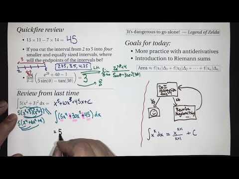
Expanding 5(x² + 3)² into 5x⁴ + 30x² + 45 makes the power rule directly applicable and gives x⁵ + 10x³ + 45x + C.
The power rule has one important exception: ∫1/t dt = ln|t|, because the usual formula would divide by zero when the exponent is −1.
The identity tan²θ = sec²θ − 1 converts the integral of (sec θ + tan θ)² into forms with known antiderivatives, producing 2tan θ + 2sec θ − θ + C.
For a(t) = 2 − 6t with v(2) = s(2) = 0, successive integration gives v(t) = 2t − 3t² + 8 and s(t) = t² − t³ + 8t − 12.
A Riemann sum on [a, b] with n equal pieces uses width Δx = (b − a)/n and approximates signed area by summing f-values at selected sample points times Δx.
Left-endpoint, right-endpoint, and midpoint choices all define valid rectangle approximations; increasing the rectangle count improves the approximation toward the integral.

Chapters

0:00 Quickfire Review: Arithmetic, Equal Partitions, and L’Hôpital’s Rule

The arithmetic check computes 13 × 11 − 7 × 14 as 143 − 98 = 45.
Dividing the interval [2, 5] into four equal pieces gives width (5 − 2)/4 = 0.75 and endpoints 2, 2.75, 3.5, 4.25, and 5.
For the limit as θ approaches 0, the 0/0 form is handled with L’Hôpital’s rule, yielding 6/2 = 3.

4:05 Antiderivatives by Expanding Polynomials and Applying the Power Rule

A useful workflow is to check whether an integrand is recognizable, rewrite it with algebra if needed, then check again.
Expanding 5(x² + 3)² gives 5x⁴ + 30x² + 45, which can be integrated term by term.
The power rule is ∫xᵏ dx = xᵏ⁺¹/(k + 1) + C for k ≠ −1; the example evaluates to x⁵ + 10x³ + 45x + C.
A single +C represents the family of antiderivatives.

13:33 Collaborative Learning and the Lecture’s Goals

Explaining a solution to a classmate can expose errors that are hard to catch in one’s own work and reinforce understanding.
The lecture’s two goals are to build fluency with antiderivatives and introduce Riemann sums as a method for finding totals.
Riemann sums initially seem separate from antiderivatives, but both are central parts of integral calculus.

16:56 Rewriting Rational Powers Before Integration

The example simplifies 12t³/t⁴ + √(t³)/t⁴ − 3t⁶/t⁴ to 12/t + t⁻⁵ᐟ² − 3t².
The power rule works for t⁻⁵ᐟ² and t², but not for 1/t because substituting k = −1 would require division by zero.
Integrating term by term gives 12 ln|t| − (2/3)t⁻³ᐟ² − t³ + C.
The integration variable can be any symbol, such as t or x, as long as the differential matches it.

23:45 Integrating (sec θ + tan θ)² with Trigonometric Identities

Known antiderivatives include ∫sec²θ dθ = tan θ and ∫sec θ tan θ dθ = sec θ.
Expanding (sec θ + tan θ)² gives sec²θ + 2 sec θ tan θ + tan²θ.
Using tan²θ = sec²θ − 1 rewrites the integrand as 2sec²θ + 2sec θ tan θ − 1.
The result is 2tan θ + 2sec θ − θ + C, with one constant covering all terms.

30:45 Initial Conditions Turn General Antiderivatives into Specific Solutions

An indefinite integral gives a family of solutions through +C; an initial condition selects a particular member of that family.
For motion, the derivative of position s(t) is velocity v(t), and the derivative of velocity is acceleration a(t).
The setup uses a(t) = 2 − 6t and the conditions v(2) = 0 and s(2) = 0 to determine the integration constants.

33:30 Finding Position and Velocity from Acceleration and Conditions at t = 2

Integrating a(t) = 2 − 6t gives v(t) = 2t − 3t² + C; applying v(2) = 0 gives C = 8.
Integrating v(t) = 2t − 3t² + 8 gives s(t) = t² − t³ + 8t + D; applying s(2) = 0 gives D = −12.
The resulting initial velocity is v(0) = 8 yards per minute, and the initial position is s(0) = −12 yards.
The acceleration’s units, yards per minute squared, are consistent with velocity in yards per minute and position in yards.

39:35 Integral Calculus Approximates Totals with Thin Rectangles

Differential calculus asks how quantities change, while integral calculus asks for totals, including signed area under a curve.
A curved region can be approximated by splitting it into thin strips and replacing each strip with a rectangle.
More rectangles generally reduce approximation error; the limiting idea is to let the number of rectangles increase without bound.

43:20 Riemann Sums: Equal Widths and Flexible Sample Points

For y = f(x) on [a, b], divide the interval into n equal subintervals, each of width Δx = (b − a)/n.
Each rectangle’s height comes from evaluating f at a chosen point in its subinterval, and its area contribution is height times Δx.
Adding the rectangle contributions approximates the signed area from a to b; the sample point may be the left endpoint, right endpoint, or midpoint.
The interval partition determines the widths, while function evaluations at the chosen sample points determine the heights.

Transcript excerpt

0:00 And we'll start with our quickfire review. First problem. If you take 13 * 11 subtract 7 * 14, what do you get? >> 45. Yes, that is the correct answer. 13 * 11 being 143 and uh 7 * 14 being 98. Now the next one, this is sort of a a foreshadow of things to come today. If you cut the interval from 2 to 5 into four smaller and equally sized pieces, where will the end points of the interval be? So just to be clear before we say the answers out loud, we're thinking of it. We are going from two to five and we're cutting into four equally

0:49 sized pieces. And four is a pretty good number to figure out how to slice. So the question is where have you put your cuts? All right. So besides two and five, those are the obvious ones. Where are the cuts happening? >> Can you say that again? >> Add 75 to each one. >> Yeah. Okay. So, so you said 2.75, 3.5, and 4.25. >> Yeah. >> Yeah. All right. Now, you might say, well, how did we get that? Well, in some sense, you can answer an

1:37 easier question, which is to say, how far is it from two to five? That's not a hard question. How far is it from two to five? >> Three. All right. So, we know how far the whole thing is. So then how far is one interval or how wide is one interval? If there's four intervals and I have to cover a distance of three, how how wide is one of them? >> Three over four, right? Three is a total distance I have to cover. I have four intervals. They're all the same size. So now I know the

This is the start of the transcript. Save this video free for the whole transcript, searchable and time-coded.

Related notes

Summary, takeaways, and chapters were generated by AI from the video's transcript and may contain errors. The video belongs to its creator, Beard Meets Calculus.