Definite integrals (Calc 1; Lecture 3-8; Fall 26)
Overview
The lecture introduces definite integrals as limits of Riemann sums that measure accumulated totals, then develops their notation, basic values, and core properties. Worked examples show how to combine known integrals, use odd and even symmetry, compute an average value, and apply the integral mean value theorem; an opening review also revisits algebra and Newton's method.
Key takeaways
- A definite integral is the limit of sums of thin rectangles, and its bounds specify where accumulation starts and stops.
- Reversing integral bounds reverses the sign, while splitting or joining adjacent intervals preserves the total when orientation is handled correctly.
- Linearity lets known integral values be combined: from ∫₁³ f=6, ∫₂³ f=7, and ∫₂⁵ f=3, one obtains ∫₁⁵ f=2.
- Symmetry can replace lengthy integration: odd functions integrate to zero over [−b,b], while even functions reduce to twice the integral over [0,b].
- The average value on [a,b] is the integral divided by interval length; continuity guarantees that the function equals this average at some point in the interval.
Chapters
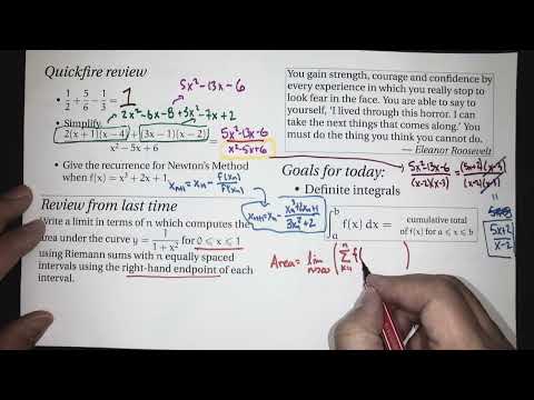
- Expands the numerator 2(x+1)(x-4) + (3x-1)(x-2) to 5x² - 13x - 6.
- Factors the expression as (5x+2)(x-3), while x² - 5x + 6 factors as (x-2)(x-3).
- Cancels the shared factor to obtain (5x+2)/(x-2), while the original expression remains undefined at x=3.
- Uses Newton's method, xₙ₊₁ = xₙ - f(xₙ)/f′(xₙ), to approximate roots.
- For f(x)=x³+2x+1, identifies f′(x)=3x²+2.
- Writes the recurrence as xₙ₊₁ = xₙ - (xₙ³+2xₙ+1)/(3xₙ²+2).
- Sets up the area on [0,1] using n equal intervals and right endpoints k/n.
- Writes the limit as limₙ→∞ (1/n) Σₖ₌₁ⁿ 1/(1+(k/n)²).
- Rewrites the sum as limₙ→∞ n Σₖ₌₁ⁿ 1/(n²+k²), emphasizing that the limit gives the exact area.
- Shares Eleanor Roosevelt's advice that facing feared tasks builds strength, courage, and confidence.
- Connects the quote to studying calculus: challenges often feel harder before starting than they prove to be in practice.
- Defines ∫ₐᵇ f(x) dx as the limit of Riemann sums, representing accumulation from x=a to x=b.
- Interprets dx as the infinitesimal-width counterpart of Δx and the integral sign as an elongated S for summation.
- Distinguishes definite integrals, whose outputs are numbers, from indefinite integrals, whose outputs are families of functions.
- Frames a definite integral as a total, with applications such as area, length, volume, money, or electrical charge.
- Reviews reference values: ∫₀ᵇ 1 dx=b, ∫₀ᵇ x dx=b²/2, ∫₀ᵇ x² dx=b³/3, and ∫₀ᵇ eˣ dx=eᵇ−1.
- Extends the examples to [a,b], including ∫ₐᵇ 1 dx=b−a and ∫ₐᵇ eˣ dx=eᵇ−eᵃ.
- Reversing the bounds changes the sign: ∫ₐᵇ f(x)dx = −∫ᵦᵃ f(x)dx; equal bounds give zero.
- Uses linearity to split sums and differences and to pull out constant factors.
- Shows that adjacent intervals combine as ∫ₐᵇ f + ∫ᵦᶜ f = ∫ₐᶜ f, with reversed orientation handling overlapping intervals.
- Bounds an integral using m≤f(x)≤M on [a,b]: m(b−a)≤∫ₐᵇ f(x)dx≤M(b−a).
- Given ∫₁³ f=6, ∫₂³ f=7, and ∫₂⁵ f=3, combines the intervals to find ∫₁⁵ f.
- Corrects the overlap on [2,3] by subtracting it: ∫₁⁵ f = 6+3−7 = 2.
- Recasts subtraction as reversed bounds, using ∫₃² f=−∫₂³ f to chain the intervals.
- For an odd function, contributions cancel on [−b,b], so ∫₋ᵦᵇ f(x)dx=0.
- For an even function, the two halves match, giving ∫₋ᵦᵇ f(x)dx=2∫₀ᵇ f(x)dx.
- Recognizes t³/(1+cos²t+t⁴) as odd because t³ changes sign while cos²t and t⁴ remain unchanged.
- Uses the odd-function rule to evaluate its integral from −5 to 5 as zero.
- Defines the average value of f on [a,b] as (1/(b−a))∫ₐᵇ f(x)dx, the height of a rectangle with matching width and area.
- For f(x)=4−x² on [0,2], computes the average as (1/2)(8−8/3)=8/3.
- States that if f is continuous on [a,b], some c in [a,b] satisfies f(c)=(1/(b−a))∫ₐᵇ f(x)dx.
- Justifies the theorem by bounding the average between the function's minimum and maximum, then using continuity to ensure the function attains that value.
Transcript excerpt
0:00 Start with our quickfire review. If we have a half add 56 subtract 1/3, what do we get? >> It is the one. All right. Good. Well, uh, next one. Simplify 2 * x + 1 * x - 4 + 3 x -1 * x - 2 all / x^2 - 5 x + 6oo. Okay. Uh well hopefully that simplifies. And what does that simplify to? Somebody work it out. >> 5 - 8x - 2. >> What was it? 5 - 8 x - 2
0:53 >> 5 - 8 over x - 2. Oh my goodness, you even did long division. Wow. Uh, okay. Let's work it out. I think you're right. I'm not going to go quite that simple. Uh, but but let's talk about it. So, this is working with our algebra. And I know you're like, "Algebra, that's an old class. I don't need to know my algebra." No, no, no. Most of calculus happens in the algebra. The calculus part is often just a few steps that happen along the way. Most of the work is algebra. So, we got to keep our algebra skills up. So, what would we do to simplify this part? The 2 * x + 1 * x - 4. you'd foil, distribute, expand, whatever
1:45 you like to call it. So from that part, if we multiply out, we'd have 2x^2. Here's a - 4x + x. That' normally be a - 3x, but there's a 2. So that makes - 6x - 4 * 2 - 8. Then you do the same thing to this part. And the good news is that you have a plus. So 3x * x 3x^2 Then we have - 6x - x. So that's - 7 x and -1 * -2 is + 2. [clears throat]
This is the start of the transcript. Save this video free for the whole transcript, searchable and time-coded.
In this course
Related notes
Summary, takeaways, and chapters were generated by AI from the video's transcript and may contain errors. The video belongs to its creator, Beard Meets Calculus.