ECircuits-Lec13-2026
Overview
The lecture derives how a single-pole op amp’s closed-loop bandwidth depends on loop gain, showing that the gain-bandwidth product is approximately conserved between open-loop and closed-loop operation. Worked examples use an inverting amplifier with 20 MHz gain-bandwidth product and an LM321 with 1 MHz gain-bandwidth product, then explain how DC biasing, coupling capacitors, and separate DC/AC analysis make practical amplifier circuits work.
Key takeaways
- For a single-pole op amp with large loop gain, closed-loop bandwidth is approximately T0fp, and closed-loop gain times bandwidth is approximately the open-loop gain-bandwidth product A0fp.
- An op amp with a 20 MHz gain-bandwidth product configured for gain 9 has an estimated closed-loop bandwidth near 2 MHz; the exact first-order expression includes a 1 + T0 factor.
- The LM321 example yields an open-loop pole near 20 Hz from its 50,000 DC gain and 1 MHz gain-bandwidth product; a feedback factor near 1/100 gives about 10 kHz bandwidth at gain 100.
- Negative feedback lets a designer exchange excess gain for bandwidth, so a high-gain op amp with limited open-loop bandwidth can support applications such as audio amplification at lower gain.
- A single-supply amplifier powered from 0 V and 5 V needs a bias point near 2.5 V to amplify small AC signals without saturating at a rail.
- In linear op amp circuits, analyze DC with capacitors open and AC with coupling capacitors shorted; this separates bias design from signal-gain analysis.
Chapters
- Homework 3 and Lab 2 are due Friday, September 25; a broken homework hyperlink was fixed.
- Exam 1 is available on Canvas and is due Friday, October 2, giving students nearly two weeks.
- The exam problems build on the techniques used in Homework 1 through 3.
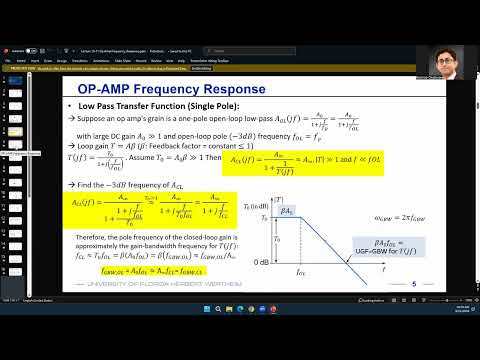
- The op amp open-loop response is modeled as A0 divided by 1 + j(f/fp), a first-order low-pass response.
- With loop gain T(f) = T0/[1 + j(f/fp)], the closed-loop response is approximately A∞/[1 + j(f/(T0fp))] when T0 is much greater than 1.
- The approximation gives a closed-loop bandwidth of about T0 times the open-loop pole frequency fp.
- The open-loop gain-bandwidth product is A0fp, while the approximate closed-loop bandwidth is βA0fp.
- Since the ideal closed-loop gain A∞ is approximately 1/β, multiplying closed-loop gain by closed-loop bandwidth recovers A0fp.
- The gain-bandwidth relationship lets designers estimate closed-loop bandwidth from an op amp datasheet and the circuit’s gain.
- The circuit has ideal inverting gain A∞ = −R2/R1 = −9 and feedback factor β = R1/(R1 + R2) = 0.1.
- With A0 = 10^5 and open-loop pole fp = 200 Hz, the open-loop gain-bandwidth product is 20 MHz.
- The approximate closed-loop bandwidth is 0.1 × 20 MHz = 2 MHz; finite open-loop gain makes the actual closed-loop gain about −8.999.
- The exact first-order bandwidth expression includes a 1 + T0 factor, while T0fp is a close approximation when T0 is large.
- The example’s loop gain begins near 10^4 and falls at approximately −20 dB per decade after the 200 Hz pole.
- The loop-gain curve crosses unity near 2 MHz, matching the estimated closed-loop bandwidth.
- Negative feedback trades excess gain for bandwidth, making a high-gain, narrow-bandwidth op amp useful as an audio amplifier when its gain is reduced.
- The LM321 model uses a DC open-loop gain of 50,000, input resistance of 1 MΩ, and output resistance of 1 kΩ.
- A unity feedback factor is specified to produce a 1 MHz closed-loop bandwidth, revealing an open-loop gain-bandwidth product of approximately 1 MHz.
- Dividing 1 MHz by the open-loop gain of 50,000 gives an open-loop pole frequency of 20 Hz.
- For the non-inverting resistor network, ideal closed-loop gain is 1 + R2/R1 = 100.
- The feedback calculation includes the LM321’s 1 kΩ output resistance, 1 MΩ input resistance, and surrounding resistors; the resulting β is approximately 1/100.
- With A0 = 50,000, the loop gain is approximately 500 and the closed-loop bandwidth is about 10 kHz.
- The 100 gain and 10 kHz bandwidth are consistent with the LM321’s approximately 1 MHz gain-bandwidth product.
- An op amp produces useful small-signal gain only when its operating point lies in the steep, central region of its voltage transfer characteristic.
- With a 0 V to 5 V supply range, a single-supply amplifier should generally be biased near 2.5 V rather than centered at 0 V.
- An inverting amplifier connected to ground without a suitable bias can saturate at a supply rail instead of amplifying its AC input.
- Dual supplies such as +5 V and −5 V can place 0 V at the middle of the available output range.
- A pair of 1 MΩ resistors between a 10 V supply and ground creates a 5 V bias point when the op amp’s high input impedance draws negligible current.
- Input and output coupling capacitors block DC because their impedance is infinite at zero frequency, while passing AC signals at sufficiently high frequencies.
- A feedback-path capacitor blocks DC current so the op amp’s positive and negative inputs can both remain at the 5 V bias point.
- Coupling capacitors isolate the amplifier’s DC operating point from external source and load voltages.
- For DC analysis, capacitors are open circuits; the divider sets the positive input to 5 V, feedback holds the negative input near 5 V, and the output rests near 5 V.
- For AC analysis, coupling capacitors are treated as shorts, reducing the circuit to a familiar feedback amplifier with resistors and an AC source.
- Superposition permits separate DC-bias and AC-signal calculations when the op amp operates in its linear region.
- If the op amp enters a nonlinear region, such as saturation, the linear superposition assumption no longer accurately predicts the combined response.
Transcript excerpt
0:02 All right. So, some of the announcements first, um, homework 3 has been posted last week already and the due date would be, uh, Friday, this week, September 25th. So, please go over the homework three problems and I think there was a problem with the hyperlink someone mentioned. I just fixed that. Um, we have also posted a few similar problems which we'll discuss today. uh very similar to your actual homework three problems that will help you solving the particular homework. Um also exam one has been uploaded um and according to the according to the original syllabus exam one was due this week as well but because this week we have homework three due as well as lab two due um I am making exam one available for the next two weeks. So submit it anytime before
0:49 October 2. So that would be next week Friday not this week. So you'll have almost two weeks. So one week plus five days to complete exam one. Um and very similar to other homework problems just uh uh provide your solutions or upload your solutions on canvas. Very similar to your homework one to three. And uh if you have solved homework one two and three most of these problems will be very easy for you to solve. So please go over there and upload it within any time before October 2. Any question on on homework exam one? So in terms of deadlines this week we have homework three as well as lab two. Those are the two things that are due
1:36 this week and next week exam one will be due. All right. So today I would like to finalize our discussion on opamp frequency response. The most important thing is listed in this slide. So which
This is the start of the transcript. Save this video free for the whole transcript, searchable and time-coded.
In this course
Related notes
Summary, takeaways, and chapters were generated by AI from the video's transcript and may contain errors. The video belongs to its creator, WISE Lab - UF ECE.