ECircuits-Lec12-2026
Overview
The lecture derives how a single-pole op-amp’s output resistance and parasitic capacitance create a low-pass response, then shows how negative feedback trades open-loop gain for closed-loop bandwidth. For a first-order amplifier, the gain-bandwidth product stays constant: an op-amp with A0 = 250,000 and a 1 MHz unity-gain frequency has a 4 Hz open-loop pole, while reducing its closed-loop gain to 1,000 raises bandwidth to about 1 kHz. The derivations are applied to 741 op-amp examples and Homework 3 calculations, including feedback factors, closed-loop pole frequencies, and the limits of the single-pole approximation.
Key takeaways
- A first-order op-amp with DC gain 250,000 and a 1 MHz unity-gain frequency has an open-loop pole near 4 Hz, because A0fp = 1 MHz.
- Negative feedback trades closed-loop gain for bandwidth: reducing gain by a factor of 250, from 250,000 to 1,000, raises bandwidth from about 4 Hz to about 1 kHz.
- For a single-pole op-amp, the closed-loop pole is approximately (A0β)fp when A0β is large, and more exactly (1 + A0β)fp.
- A unity-gain buffer with β = 1 exposes the op-amp’s unity-gain frequency as its closed-loop bandwidth; the lecture’s 741 example yields about 20 MHz.
- Gain-bandwidth constancy depends on the single-pole response; a second pole changes the roll-off slope and invalidates the simple gain-times-bandwidth rule.
- In the 1 kΩ/9 kΩ inverting example, β = 0.1 implies an approximate gain magnitude of 10, but KCL gives the exact signed gain −9.
Chapters
- Homework 3 on op-amp frequency response is due the following Friday, with two similar practice problems posted on Canvas.
- Lab 2 prelab and in-lab materials are available, and the first take-home test will be posted Sunday night with about 10 days to complete.
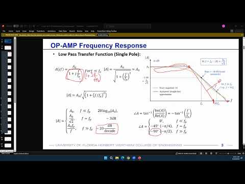
- An op-amp’s output resistance combines with output-node parasitic capacitance to create an RC low-pass pole.
- For a first-order response, the transfer function is A0/(1 + jf/fp), where fp is the pole frequency and A0 is the DC gain.
- Below fp, the gain magnitude is approximately A0; at fp, it falls to A0/√2, the minus-3 dB point.
- Above fp, one pole produces a minus-20 dB-per-decade gain slope and phase approaches minus 90 degrees, passing through minus 45 degrees at fp.
- For a first-order system, the unity-gain frequency equals the gain-bandwidth product; this equivalence does not generally hold for a two-pole system.
- With a single-pole op-amp, loop gain varies with frequency as T(f) = T0/(1 + jf/fp), where T0 = A0β.
- The closed-loop gain follows A0/(1 + 1/T(f)), extending the familiar low-frequency feedback relation to frequency-dependent loop gain.
- For large T0, the closed-loop response is approximately Aideal/(1 + jf/(T0fp)), so the closed-loop pole is about T0 times the open-loop pole.
- The closed-loop low-frequency gain is approximately 1/β, while the bandwidth rises as feedback reduces the gain.
- More exactly, the closed-loop pole is (1 + T0)fp; using T0fp is a close approximation when loop gain is large.
- A 741 example uses a 1 MHz unity-gain frequency and an open-loop DC gain of 250,000, giving an open-loop pole near 4 Hz.
- Reducing closed-loop gain from 250,000 to 1,000 increases bandwidth by about 250 times, from 4 Hz to 1 kHz.
- A closed-loop gain of 100 would allow roughly 10 kHz bandwidth, illustrating the gain-bandwidth tradeoff for audio-range applications.
- For an op-amp with A0 = 100,000, open-loop pole f1 = 200 Hz, and gain-bandwidth product of 20 MHz, a 1 kΩ and 9 kΩ feedback network gives β = 0.1.
- The ideal closed-loop gain magnitude is 1/β = 10, and the loop gain is T0 = A0β = 10,000.
- The closed-loop pole is approximately βA0f1 = 2 MHz, ten times the open-loop gain-bandwidth product multiplied by β.
- With β = 1, the same A0 = 100,000, f1 = 200 Hz op-amp has an approximately 20 MHz closed-loop bandwidth and unity gain.
- Homework 3 provides op-amp input resistance, output resistance, and DC gain, then asks for closed-loop quantities across feedback configurations.
- When β = 1, the stated closed-loop bandwidth directly identifies the op-amp’s unity-gain frequency under the single-pole assumption.
- The feedback relation Aclosed = Aopen/(1 + βAopen) reduces to approximately 1/β when the open-loop gain and T0 are large.
- For β = 1, closed-loop bandwidth is approximately A0 times the open-loop pole frequency, which is the unity-gain frequency for a single-pole op-amp.
- The assignment’s 2 MHz bandwidth at β = 1 therefore specifies a 2 MHz unity-gain frequency; the requested closed-loop pole is approximately T0fp, or exactly (1 + T0)fp.
- A similar problem gives a 1 MHz bandwidth at β = 1, so the single-pole op-amp’s gain-bandwidth product is 1 MHz.
- For β = 1/31.5, the ideal closed-loop gain is 31.5 and the estimated bandwidth is 1 MHz/31.5, or about 32 kHz.
- The lecture emphasizes that open-loop and closed-loop gain-bandwidth products match only for a first-order system.
- For the inverting 1 kΩ/9 kΩ circuit, KCL gives a signed gain of −9; using 1/β = 10 gives an approximate magnitude with about 10% error.
- β describes the feedback fraction, not whether feedback is positive or negative; the circuit connection determines the sign of the closed-loop gain.
- For high loop gain, T0fp is an acceptable closed-loop-pole estimate, while (1 + T0)fp is the more exact expression.
Transcript excerpt
0:01 Okay. Uh so today we are mostly going to discuss about the uh frequency response of an amplifier specifically opamps. Um also please note that your homework 3 has also been uploaded on canvas. The due date would be next Friday. Um however like this homework three deals with frequency response of opamps and um that is something that we're going to discuss today. So only after today's class you'll probably have a good idea about how to solve homework three problems. uh however I have also uploaded two similar problems as homework 3 which would help you to understand what we are actually looking for and how we are trying to solve homework three problems. So um that is one thing and then the second announcement is that your lab two which is due next week um is also uploaded the
0:52 prelab as well as the inlab sections. Uh along with this, we'll also have our first take-home test. Um I'll upload the questions Sunday night at um at 12:00. Um and I'll give you about 10 days because I think there are multiple things next week. There is the lab, there is the uh homework three. So I I'll give a little bit more time to complete the take-home test. And the takeh home test would be very similar to any of the other assignments, homework assignments. Just like you have uploaded your homework one, homework two and homework three, your take-home test will look very similar. It will just be a set of questions that you need to solve and upload on canvas. So it would be very similar to any of the other homework assignments that you have already completed. Uh and I'll provide a little bit extra time. I know in syllabus it is
1:39 written to be one week but I'll provide
This is the start of the transcript. Save this video free for the whole transcript, searchable and time-coded.
In this course
Related notes
Summary, takeaways, and chapters were generated by AI from the video's transcript and may contain errors. The video belongs to its creator, WISE Lab - UF ECE.