ECircuits-Lec14-2026
Overview
The lecture develops small-signal op-amp analysis by separating AC and DC with superposition, using capacitor behavior to simplify each analysis, and biasing the amplifier near 5 V on a 0 to 10 V supply. It then applies RC filter analysis and the open-circuit time-constant method to estimate how C1, C2, and C3 set low-frequency poles, including a 50 Hz design target and an estimated 1 to 5% approximation error.
Key takeaways
- For a linear op-amp operating with small signals, AC and DC can be analyzed separately using superposition, which turns a complicated circuit into separate bias and signal models.
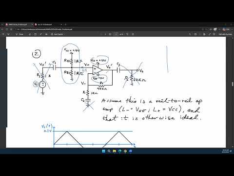
- With a 10 V supply and equal 1 MΩ bias resistors, the non-inverting input is set to 5 V; negative feedback and zero DC current through R2 bring the inverting input and output to approximately 5 V as well.
- A capacitor's DC model is an open circuit, while its high-frequency model approaches a short; the RC cutoff determines whether either approximation is appropriate for the signal frequencies of interest.
- For C1's input high-pass network, calculate the resistance across the capacitor with independent sources zeroed, then use f_c = 1/(2πR_eqC1) to design the 50 Hz corner.
- The open-circuit time-constant method estimates one pole at a time by opening the other capacitors; it is convenient for multi-capacitor circuits but may differ from exact analysis by roughly 1 to 5% in the example.
- Checking a capacitor's circuit at ω = 0 and ω → ∞ is a direct way to identify whether its network behaves as a high-pass, low-pass, or another filter.
Chapters
- Superposition applies when the op-amp operates linearly, with a constant gain over the signal amplitudes and bandwidth being analyzed.
- Large inputs can push an op-amp into nonlinear operation or saturation; the lecture focuses on small signals instead.
- Treating AC and DC sources separately reduces a combined circuit to simpler bias and signal analyses.
- For DC, a capacitor is an open circuit because its impedance 1/(jωC) becomes infinite at ω = 0.
- A first-order RC low-pass has transfer function 1/(1 + jωRC), with its -3 dB cutoff at ω = 1/RC.
- At frequencies well above the RC cutoff, the capacitor approaches a short; whether a short or open approximation is useful depends on the frequency range of interest.
- With capacitors open for DC, C1 and C2 disconnect the AC source, ground path, and load from the bias calculation.
- Equal 1 MΩ resistors RB1 and RB2 divide a 10 V supply to establish 5 V at the non-inverting input.
- Negative feedback makes the inverting input approximately 5 V; with no DC current through R2, the output is also approximately 5 V.
- Biasing near the midpoint of the 0 to 10 V range keeps the amplifier in a region where small input changes can produce gain.
- For AC analysis, fixed DC supplies such as the 10 V VCC are AC ground because they do not fluctuate.
- Capacitors that pass the frequencies of interest are modeled as shorts, while DC bias values are omitted from the small-signal circuit.
- RB1 and RB2 may connect the signal node to AC ground, but with an ideal op-amp's infinite input impedance they do not divide the voltage at its input.
- A finite op-amp input impedance or significant source resistance can create voltage division and must be included.
- The design task sets a lower -3 dB frequency of 50 Hz for the circuit's high-pass response.
- C1 is in series with the input, and the resistance on its far side provides a path to ground, creating a high-pass RC network.
- The cutoff is f = 1/[2π(RS + RX)C1] when the capacitor sees source resistance RS and effective load resistance RX.
- Find the resistance seen across C1 by zeroing independent sources, then choose C1 to meet the 50 Hz cutoff.
- For the example, C1 sees RS in series with RB1 || RB2; the parallel bias resistance is approximately 501 kΩ.
- Use 1/(2πRC) = 50 Hz with C1's equivalent resistance to calculate its capacitance.
- For C2, short the AC input and use the op-amp's virtual-ground behavior to find an effective resistance of R1, given as 1 kΩ.
- The resistance seen by a capacitor is found by looking into its terminals with independent sources zeroed and circuit constraints accounted for.
- The open-circuit time-constant method analyzes one capacitor at a time while treating the other capacitors as open circuits.
- For C3, the ideal op-amp output resistance is zero, and the approximation leaves the 50 kΩ load RL as the principal resistance seen by the capacitor.
- The method avoids a more complicated multi-capacitor pole calculation, but it estimates rather than exactly determines the circuit response.
- Each capacitor's approximate time constant is RC, which gives a corresponding pole near 1/RC in angular frequency.
- Ignoring other capacitors can change the result when those capacitors create additional current paths, especially in the C3 calculation.
- For the discussed circuit, the instructor estimates typical OCTC error at roughly 1 to 5%; an estimated 50 Hz pole might be about 47 or 53 Hz in a more exact result.
- An ideal op-amp's zero output impedance can make some parallel paths disappear, while a nonzero example such as 100 Ω can change the resistance calculation.
- Use simulation or measurement when an exact pole location is required.
- To identify a capacitor's filtering effect, compare the circuit limits at ω = 0, where the capacitor is open, and ω → ∞, where it is short.
- Applying those two limits to C2's surrounding R1 and R2 network reveals its frequency-dependent behavior.
- C1 and C3 are series-path capacitors with resistive paths to ground, so each contributes a high-pass response.
- C1, C2, and C3 each contribute a pole; setting all three near 50 Hz creates a much steeper combined low-frequency rolloff than separating their poles.
- One capacitor can set the 50 Hz corner while the others are assigned lower corners, such as 5 Hz, to separate their effects.
- The capacitor values are not unique: choosing C1, C2, or C3 for the 50 Hz target is valid if the remaining values are recalculated accordingly.
- The next topic is diodes and how nonlinear device behavior, alongside BJT and MOSFET nonidealities, contributes to practical op-amp limitations.
Transcript excerpt
0:00 Yeah. >> So we have been discussing this particular problem uh which is very similar to your homework 3. Um and uh in the last lecture as we discussed that we are going to sort of look into the AC and DC differently because you can always consider your AC signals or AC voltages and currents as one type of source and your DC signals DC voltages and currents as another type of source. Now because superposition principle will hold true for any linear circuit and assuming that the OPM is linear last class there was a question that what happens if the OPM is not linear not not in the linear detail then of course the superposition principle will not be true or will not be fully true depending on how much nonlinear you are right but we are not going into that much details or
0:49 that much advanced analysis of the circuits we're assuming that the opamp is still linear that means it provides a gain which is always the same. The gain does not always the same in the sense that uh depending on the the u amplitude of the input you're going to get a gain that is a times or you're going to get an output which is a times the input and that value of a is going to be a constant value um of course up to the certain bandwidth. So below that bandwidth that gain is going to be constant. Now what happens in a nonlinear regime of operation is that as you as you are changing the input amplitude if you have a very small amplitude you'll probably have a gain that is um let's say a * for this particular op and the
1:39 output is going to be a * the input and
This is the start of the transcript. Save this video free for the whole transcript, searchable and time-coded.
In this course
Related notes
Summary, takeaways, and chapters were generated by AI from the video's transcript and may contain errors. The video belongs to its creator, WISE Lab - UF ECE.