NDSU ECE 211 Lecture 28
Overview
Roger Green derives Euler's formula, e^(jθ) = cos θ + j sin θ, from the Taylor series and uses it to explain complex exponentials as rotating unit vectors. He defines phasors as complex vectors encoding a sinusoid's peak amplitude and phase, then demonstrates how equal-frequency sinusoids can be added by adding phasors, verifying the result in MATLAB with a 3 cos(10t + 45°) minus 2 cos(10t - 60°) example.
Key takeaways
- Euler's formula, e^(jθ) = cos θ + j sin θ, follows by substituting jθ into the exponential's Maclaurin series and grouping real and imaginary terms.
- A complex exponential e^(j(ωt + θ)) has unit magnitude and rotates counterclockwise when ω is positive; its real part is cos(ωt + θ).
- A phasor stores a sinusoid's peak amplitude and phase while leaving its known frequency implicit.
- Adding sinusoids with different phases is a phasor-addition operation only when they share the same frequency; sine terms must first be converted to cosine form.
- For 3 cos(10t + 45°) − 2 cos(10t − 60°), phasor addition gives an equivalent sinusoid of approximately 4.0132 cos(10t + 1.2876), with phase in radians.
- Converting phasors to rectangular form allows direct addition of real and imaginary components, after which magnitude and phase recover the equivalent sinusoid.
Chapters
- The lecture introduces phasors as a way to simplify sinusoidal steady-state analysis.
- A Taylor series represents a function as an infinite sum of derivatives evaluated at an expansion point.
- For e^x, every derivative is e^x, so the Maclaurin series is 1 + x + x²/2! + x³/3! + continuing terms.
- Substituting jθ for x in the exponential series produces alternating real and imaginary terms because j² = -1.
- Grouping real terms yields the Maclaurin series for cos θ; grouping terms containing j yields j sin θ.
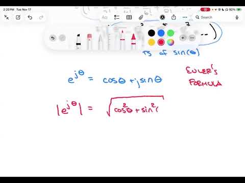
- The resulting identity is Euler's formula: e^(jθ) = cos θ + j sin θ.
- Euler's formula gives |e^(jθ)| = √(cos² θ + sin² θ) = 1.
- In the complex plane, e^(jθ) is a unit-length vector at angle θ from the positive real axis.
- Its real and imaginary coordinates are cos θ and sin θ, respectively.
- For e^(j(ωt + θ)), the vector's angle changes with time; positive ω produces counterclockwise rotation.
- Taking the real part recovers the cosine: cos(ωt + θ) = Re{e^(j(ωt + θ))}.
- The imaginary part similarly gives sin(ωt + θ), linking rotating complex vectors to sinusoidal signals.
- A MATLAB animation plots the real and imaginary parts of a complex exponential and shows its path on the unit circle.
- The real-part plot follows a cosine waveform, while plotting both components against time creates a helix.
- The demonstration confirms unit magnitude and counterclockwise rotation for the example e^(j2πt).
- For v(t) = V₁ cos(ωt + θ₁), the phasor is V₁∠θ₁, a complex-plane vector encoding peak amplitude and starting phase.
- The phasor notation omits ω because the frequency is assumed known and shared by the signals being analyzed.
- A sine-form signal should be converted to cosine form first, using sin(a) = cos(a − 90°), or a − π/2 radians.
- Phasor addition applies to sinusoids with the same frequency, whose sum can be represented as one sinusoid.
- For A cos(ωt + θ₁) + B sin(ωt + θ₂), convert the sine term to B cos(ωt + θ₂ − 90°).
- Euler's formula rewrites each cosine as the real part of a complex exponential, preparing the terms for phasor addition.
- Factoring out the common e^(jωt) leaves the time-independent phasors A∠θ₁ and B∠(θ₂ − 90°).
- Adding those vectors produces a resultant C∠θ₃, which converts back to v(t) = C cos(ωt + θ₃).
- The method replaces manipulation of time-varying functions with addition of two complex constants.
- The example begins with v(t) = 3 cos(10t + 45°) − 2 cos(10t − 60°), with both terms at angular frequency 10.
- The negative amplitude becomes a positive amplitude by adding 180° to its phase, giving 2 cos(10t + 120°).
- The corresponding phasors are 3∠45° and 2∠120°, which are converted to rectangular form using Euler's formula.
- Rectangular components sum to approximately 1.1213 + j3.8534, yielding magnitude 4.0132 and phase 1.2876 radians, or 73.78°.
- The equivalent signal is approximately 4.0132 cos(10t + 1.2876), preserving the original angular frequency.
- MATLAB compares this analytic result with point-by-point addition of the original signals; the difference is only about 10⁻⁴ from numerical roundoff.
Transcript excerpt
0:01 Welcome to NDS issue BCE211. This is lecture 28. Last time we did a review of sinosoids talked about average power and also rip mean square or RMS values of signals. Today um we're going to talk about a concept called phasers. Uh phasers are going to be a convenient and powerful tool for us to look at this problem of sinosoidal steady state analysis. Um so let's just go ahead and jump right into it. So, we're going to be looking at what are called phasers. I will say that um I'm going to deviate deviate a little bit from the book. Uh so, you should be reading along. Uh but I will I will take my own way on this one. Uh and by and large, it's the same material. Um certainly the phaser
0:48 concept itself is the same. I just uh like a little different way of of driving it out. So phasers uh phasers are going to be a concept like I said that is going to help us in working with the syosoidal steady state analysis and really uh to understand phasers uh to understand this idea of a phaser to understand a phaser understand a phaser um we need we need to understand need to understand complex exponentials Um with a math prerex in this class um you should have seen a complex exponential before. Exponentials um you should have seen a complex
1:35 exponential before. You should have been introduced um for example to this idea of Oilers's form which relates a complex exponential to uh trig functions. Um but just to make sure we're all on the same page, I'm going to go ahead and uh just uh quickly catch us up on that. Um so let's go ahead and think uh about um
This is the start of the transcript. Save this video free for the whole transcript, searchable and time-coded.
In this course
Related notes
Summary, takeaways, and chapters were generated by AI from the video's transcript and may contain errors. The video belongs to its creator, Roger Green.