NDSU ECE 211 Lecture 26
Overview
The lecture works through an RL circuit driven by a decaying current source, reducing the network to a Thevenin equivalent with a 10e^-2t V source, 5 Ω resistance, and 0.5 H inductor. It derives the inductor response, then uses MATLAB to generate source data and plot the response, and CircuitLab to check the simulation against the analytical behavior. The transcript’s later stated current and voltage coefficients conflict with its own particular-solution calculation and 1 A initial condition; the consistent expressions are iL(t) = 2.5e^-2t - 1.5e^-10t A and vL(t) = -2.5e^-2t + 7.5e^-10t V.
Key takeaways
- A Thevenin reduction makes the inductor see a 10e^-2t V source in series with 5 Ω, giving a 0.1 s time constant for the 0.5 H inductor.
- The circuit’s natural mode decays as e^-10t, five times faster than the driving source’s e^-2t mode, so plotting only five circuit time constants does not show the source-driven tail reaching zero.
- For the stated source, circuit, and 1 A initial current, the consistent response is iL(t) = 2.5e^-2t - 1.5e^-10t A and vL(t) = -2.5e^-2t + 7.5e^-10t V.
- The transcript’s later expressions, 5e^-2t - 3e^-10t for current and -5e^-2t + 15e^-10t for voltage, are inconsistent with both its calculated particular coefficient of 2.5 and its specified initial current of 1 A.
- MATLAB can export thousands of sampled time-current pairs to CircuitLab, where a finely sampled piecewise-linear source approximates the exponential input.
- CircuitLab’s response and the source value at 0.5 s provide practical checks: the inductor starts at 1 A and 5 V, while the input source is still about 0.736 A.
Chapters
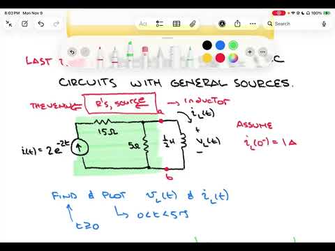
- The example uses a 2e^-2t A current source, a 15 Ω series resistor, a 5 Ω branch resistor, and a 0.5 H inductor.
- The target quantities are inductor current and voltage for t ≥ 0, with an initial inductor current of 1 A.
- The requested plots cover five circuit time constants.
- Removing the inductor leaves the source current flowing through the 15 Ω and 5 Ω resistors in series.
- The open-circuit voltage across the inductor terminals is 5(2e^-2t) = 10e^-2t V.
- Turning off the independent current source means opening it; the 15 Ω branch is disconnected, leaving Rth = 5 Ω.
- The equivalent circuit has τ = L/Rth = 0.5/5 = 0.1 s.
- The natural response decays as e^-10t, while the applied source decays as e^-2t, so the source decays five times more slowly.
- Five circuit time constants span 0.5 s, which is not long enough for the slower source-driven response to approach zero.
- KVL for the Thevenin circuit gives 10e^-2t = 5iL + 0.5 diL/dt.
- Dividing by 5 yields 2e^-2t = iL + 0.1 diL/dt, matching the general RL form f(t) = i(t) + τ di/dt.
- Using a particular-solution form A e^-2t gives A = 2.5, so ip(t) = 2.5e^-2t A.
- The complementary response has the natural form k e^-10t because τ = 0.1 s.
- Applying iL(0) = 1 A to 2.5 + k = 1 gives k = -1.5 and iL(t) = 2.5e^-2t - 1.5e^-10t A.
- Using vL = 0.5 diL/dt gives vL(t) = -2.5e^-2t + 7.5e^-10t V.
- The transcript later reports coefficients of 5 and -3 for current, which do not satisfy the derived particular solution or the stated initial condition.
- The workflow is to find a Thevenin or Norton equivalent, derive the first-order RL equation, and combine particular and complementary responses.
- The forcing function determines the particular-response shape, while the 1 A initial condition sets the complementary-response coefficient.
- The MATLAB and CircuitLab checks are intended to visualize and independently verify the response.
- MATLAB creates evenly spaced time points from 0 to 0.5 s in steps of 0.0001 s, producing about 5,001 samples.
- At each time point, the script evaluates the source current 2e^-2t and formats time-current pairs for copying.
- CircuitLab accepts the pairs as a piecewise-linear current source; the fine sampling approximates the exponential closely.
- The MATLAB script evaluates the derived inductor-current and voltage expressions across the 0 to 0.5 s interval.
- The plotted current starts at 1 A, rises to roughly 1.5 A, then falls to just under 1 A by 0.5 s.
- The voltage starts at 5 V, falls to around -1 V, and turns back toward zero; both responses combine a fast e^-10t term and a slower e^-2t term.
- The CircuitLab circuit recreates the 15 Ω resistor, 5 Ω branch, 500 mH inductor, and sampled exponential current source.
- A separate 1 A source and switch establish the inductor’s pre-switch DC current at 1 A.
- An additional resistor gives the current source a path after switching, avoiding a dangling current-source connection.
- The time-domain simulation runs from 0 to 0.5 s with a 0.001 s step and plots the inductor voltage and current.
- The simulated traces show the expected starting values and overall shapes: current begins at 1 A and voltage at 5 V.
- The current source falls from 2 A to about 0.736 A at 0.5 s, consistent with 2e^-2(0.5), confirming that it has not yet decayed to zero.
Transcript excerpt
0:01 Welcome to IND issue EC211. This is lecture 26. Last time we laid the foundations for RL and RC circuits with general sources. Today we're going to finish that topic out by going through a um example to show how the process. Once we get the example done on paper, we'll uh use mat lab to help visualize our results and also create the data necessary to do a circuit lab simulation. So, let's take a look at a circuit um that can help us put together this idea of general sources. I'm going to take a circuit that has a current source and we'll go ahead and label that current source as if I'm going to let that current be not a
0:49 typical one. It's going to be something different. It's going to be an exponential shaped U. I'm gonna let that current IF be equal to 2 E to the minus 2T. So, it's a decaying exponential current source. I'm going to go ahead and let that current feed into a resistor. So, I'm going to have a resistor that it first runs into. Um, that resistor I'm going to let have a value of 15 ohms. And then it's going to come to a branch point to split. And on one side of that split, we're going to go through another resistor. And that's going to create our first loop here. So, we'll go ahead and put that loop in. And that uh resistor that goes down, I'll let it be 5 ohms. And then as I continue off to the right, I'll make another loop. Um, and on the other side of that, I will put an inductor. And that inductor, I'm going to have it
1:37 be a value of 1/2 Henry. And of course, like any component, it has some voltage
This is the start of the transcript. Save this video free for the whole transcript, searchable and time-coded.
In this course
Related notes
Summary, takeaways, and chapters were generated by AI from the video's transcript and may contain errors. The video belongs to its creator, Roger Green.