NDSU ECE 211 Lecture 21
 Watch on YouTube →
Overview
Roger Green derives the series and parallel equivalent-inductance rules, then applies them to a three-terminal network whose measured pairwise inductances of 50, 100, and 70 mH imply individual inductors of 10, 40, and 60 mH. He verifies the resulting 34 mH equivalent in CircuitLab, derives the op-amp integrator relationship, and closes with a practical inductor model and suggested reading on linearity and duality.
Key takeaways
- For uncoupled ideal inductors, series equivalents add directly: LEQ = ΣLi.
- Parallel ideal inductors combine by reciprocal sum, 1/LEQ = Σ(1/Li), matching the parallel-resistor formula.
- Pairwise inductance measurements of 50, 100, and 70 mH for a three-branch star network uniquely yield LA = 10 mH, LB = 40 mH, and LC = 60 mH.
- Shorting the B-C terminals makes the 40 mH and 60 mH branches parallel, or 24 mH, and then series with 10 mH, giving 34 mH overall.
- Applying a 1 A/s current ramp to an inductor makes its voltage numerically equal to its inductance in compatible units, enabling the CircuitLab check of 34 mH.
- An ideal inverting op-amp with input resistor RI and feedback capacitor CF integrates its input with gain factor -1/(RI CF), while the initial capacitor voltage contributes an output offset.
Chapters
- For three series inductors, the same current I flows through L1, L2, and L3.
- Kirchhoff's voltage law gives V = V1 + V2 + V3; substituting V = L dI/dt for each component yields LEQ = L1 + L2 + L3.
- Series inductors combine like series resistors, unlike capacitors in series.
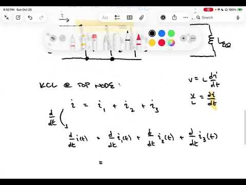
- Three parallel inductors share voltage V, while their branch currents sum to I according to KCL.
- Differentiating I = I1 + I2 + I3 and using dI/dt = V/L gives 1/LEQ = 1/L1 + 1/L2 + 1/L3.
- The reciprocal-sum rule matches the equivalent-resistance rule for parallel resistors.
- The example connects LA, LB, and LC at a hidden central node, exposing only terminals A, B, and C.
- Pairwise measurements give LAB = 50 mH, LBC = 100 mH, and LAC = 70 mH.
- Each terminal-pair measurement sees two inductors in series; the third branch is open-ended and does not contribute.
- The measurements produce three equations: LA + LB = 50 mH, LB + LC = 100 mH, and LA + LC = 70 mH.
- Roger Green represents the system as a 3-by-3 linear equation and solves it using MATLAB.
- The inferred values are LA = 10 mH, LB = 40 mH, and LC = 60 mH; their pairwise sums reproduce all three measurements.
- Shorting B and C creates terminal S, placing LB = 40 mH in parallel with LC = 60 mH.
- The parallel pair is 40 × 60 / (40 + 60) = 24 mH; it is in series with LA = 10 mH.
- The equivalent inductance from A to S is therefore 34 mH; the product-over-sum shortcut applies to two parallel elements.
- The CircuitLab test uses the 10, 40, and 60 mH inductors with B and C shorted together.
- A CSV current source ramps from 0 A at 0 seconds to 1 A at 1 second, creating dI/dt = 1 A/s.
- Since V = L dI/dt, the simulated voltage is 34 mV, confirming the calculated 34 mH equivalent.
- The inverting op-amp circuit has an input resistor RI, a feedback capacitor CF, and its non-inverting input grounded.
- The ideal op-amp draws no input current, so the resistor current equals the capacitor current; the inverting node is a virtual ground.
- Applying KCL and iC = CF dVC/dt leads to an integral relationship between the input voltage and the capacitor voltage.
- Because VC = -Vout, the output is Vout(t) = -1/(RI CF) ∫₀ᵗ Vin(τ)dτ - VC(0).
- The circuit produces a scaled, inverted integral of Vin; choosing 1/(RI CF) = 1 makes the integral scale factor unity.
- A more realistic inductor model can include series resistance RS, parallel resistance, and parallel capacitance, which are neglected when parasitics are insignificant.
- Roger Green recommends reading section 7.4 on linearity and section 7.6 on duality, while noting they are not major class-emphasis topics.
- The next topic is chapter 8, covering transient behavior in RC and RL circuits.
Transcript excerpt
0:01 Welcome to NDSU ECE211. This is lecture 21. Last time we introduced ideal conductors. We developed their current and voltage relationships. Talked a little bit about energy and power through inductors and then did some examples um using that ideal voltage current relationship that we had developed. Today we're going to continue our discussion of inductors. And like we did for capacitors, I'd like to talk about inductors in combination. So let's just run through inductors in combination. This is just another tool. Um when we have circuits that have potentially uh multiple inductors um much like when we had multiple resistors or capacitors, um
0:49 certain combinations can be reduced into fewer um equivalent inductors. and that can help assist or make simpler our analysis. So the first one I'm going to deal with are inductors in series. So we'll deal with inductors. Inductors series. If you remember when we did capacitors in series, that was the kind of hard one. It was capacitors in parallel that were the easy case where we added them. In this case, we're just going to work with inductors in series first. And I'm going to I'm going to approach this much like we did with the capacitor base. I'm going to go ahead and look at a particular source voltage. And that's going to go into a circuit that's made out of we're going to use three for right now. Three is a reasonable number. We can generalize
1:38 it higher than that later on. So we'll go ahead and show three inductors and they're all in series. We're going to go and have the first one have some inductance one and then the second one inductance 2 L2. And the last one's going to be some inductance L3. Every one of these will have a voltage um
This is the start of the transcript. Save this video free for the whole transcript, searchable and time-coded.
Related notes
Summary, takeaways, and chapters were generated by AI from the video's transcript and may contain errors. The video belongs to its creator, Roger Green.