NDSU ECE 211 Lecture 25
Overview
Roger Green explains a first-order method for analyzing RC and RL circuits with one capacitor or inductor, multiple sources, and multiple resistors: reduce the surrounding network to a Thevenin or Norton equivalent, then solve a standard differential equation. The total response combines a particular solution shaped by the forcing function and its derivatives with a complementary exponential response set by the initial condition.
Key takeaways
- A first-order RC or RL network with multiple resistors and sources can be reduced at the energy-storage element's terminals to a Thevenin or Norton equivalent.
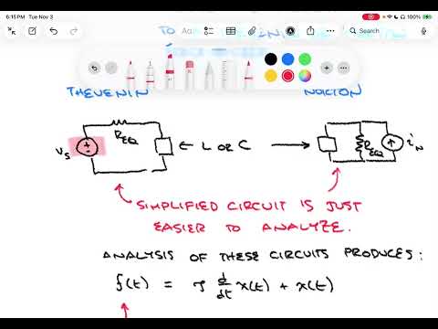
- The standard equation f(t) = τ dx(t)/dt + x(t) captures the behavior of the circuit quantity of interest, with τ determined by the reduced circuit.
- Construct a particular-solution trial by including the forcing function and the distinct terms its derivatives produce; for t sin(ω₀t), that can require as many as four components.
- For sinusoidal forcing, a trial containing both sine and cosine terms lets substitution determine the steady-state amplitude and phase through coefficient matching.
- The source-free complementary response is exponential, K e^(−t/τ), and its constant K is fixed by the initial condition.
- Because the circuit is linear, the total response is the sum of the particular, source-driven response and the complementary, natural response.
Chapters
- The lecture builds on source-free and DC-driven RL circuits from the previous lesson.
- The method covers first-order systems with exactly one energy-storage element, either a capacitor or an inductor.
- The expanded circuits may include multiple sources and resistors, while retaining a single capacitor or inductor.
- Temporarily set aside the capacitor or inductor and view the remaining sources and resistors as a two-terminal network.
- Replace that network with a Thevenin voltage source and series resistance, or a Norton current source and parallel resistance.
- The equivalent reduces a network with many resistors to a familiar single-source, single-resistance RC or RL circuit.
- The circuit quantity of interest follows the form f(t) = τ dx(t)/dt + x(t), where τ is the circuit time constant.
- For an RC circuit, x(t) is often capacitor voltage; for an RL circuit, it is often inductor current.
- The forcing term f(t) is related to the applied source and circuit values, and becomes zero when there is no driving source.
- Candidate inputs include exponentials e^(st), constants, sinusoids, and inputs multiplied by t, such as t e^(st) or t sin(ω₀t).
- A particular-solution trial includes the forcing function and any new terms produced by differentiating it.
- For example, t e^(st) requires t e^(st) and e^(st) terms, while a sinusoid requires both sine and cosine terms.
- For a cosine forcing function, use a trial solution xₚ(t) = A cos(ω₀t) + B sin(ω₀t).
- Substitute the trial into f(t) = τ dx/dt + x and determine A and B by matching the sine and cosine terms.
- The resulting particular response is the sustained, steady-state contribution associated with the continuing sinusoidal input.
- Setting f(t) = 0 gives the homogeneous equation, whose first-order solution is x꜀(t) = K e^(−t/τ).
- The complementary solution is also called the homogeneous solution and represents the circuit's natural response to stored energy.
- Linearity lets the complete response be written as x(t) = xₚ(t) + x꜀(t), combining the forced and natural contributions.
- The remaining unknown in the complementary term is K, found by applying the capacitor-voltage or inductor-current initial condition.
- The lecture frames the method as divide and conquer: solve the source-driven particular response, solve the source-free complementary response, then add them.
- Lecture 26 is planned as a full worked RC or RL example with a generalized source and potentially multiple resistors.
Transcript excerpt
0:01 Welcome to ECE 211. This is our 25th lecture. Last time we were considering circuits with resistors and a single inductor. And we looked at the transient responses under two conditions. One was a source-free case where the initial condition of the inductor drove the circuit response. And the second one was a more general case where we allowed a DC source to also be included in the circuit. In that case, the DC source could cause a response through that RL network. And it also had the possibility of having a component from an initial condition on that inductor as well. Today, we're going to lay down the foundation um for a more general solution to RC and RL circuits. We've
0:49 looked at RC and RL separately. Um we know that they both have similar forms. Um we're going to spend our time focusing now on generalizing the type of source and also looking at what happens when you have multiple resistors, for example, um and how you might approach a problem or circuit that has that added complexity. So, we're going to just do basically the foundations. We're going to do the foundations for foundations foundations for RC and RL circuits. Right? With general, what are called general sources. These aren't fully generalized, but they're more general than we've
1:37 treated up to this point. So, general sources. Um it will take a little while to lay out the um approach here. And so, today we'll lay out the approach. We'll get an idea of what's involved in the process for uh getting the solution carried out. And it will be the next lecture that we will do a really detailed example. That entire next lecture, lecture 26, will be a single example um showing how to solve an RL or an RC circuit for a general
This is the start of the transcript. Save this video free for the whole transcript, searchable and time-coded.
In this course
Related notes
Summary, takeaways, and chapters were generated by AI from the video's transcript and may contain errors. The video belongs to its creator, Roger Green.