ME2120-002
Overview
Ryan C. Cooper extends a pendulum analysis from angular motion to Cartesian position, velocity, cable tension, and energy, comparing linear and nonlinear models. The examples show why large-angle linearization can misrepresent energy and design loads, and how quantitative curve comparisons and engineering judgment support safer decisions.
Key takeaways
- A pendulum’s Cartesian velocity can be visualized with a quiver plot; vectors are largest at the bottom of the swing and smallest near its turning points.
- Cable design should use dynamic tension derived from the pendulum’s motion, not only a static load estimate; speed and centripetal acceleration affect the force near the bottom of the arc.
- For a gravity pendulum, potential energy relative to the bottom is mgL(1 − cos theta), while kinetic energy is based on the square of tangential speed.
- The small-angle approximation replaces sine theta with theta and effectively turns the pendulum into a spring-like system with quadratic potential energy, unlike the actual cosine-shaped gravitational potential.
- Model comparisons are more useful when expressed quantitatively: Cooper’s 60-degree example gives periods of about 2.7 seconds for the linear model and 2.9 seconds for the nonlinear model.
- Numerical integration can add overshoot and undershoot as each time step advances the solution; this discretization error is distinct from the physical modeling error caused by linearization.
Chapters
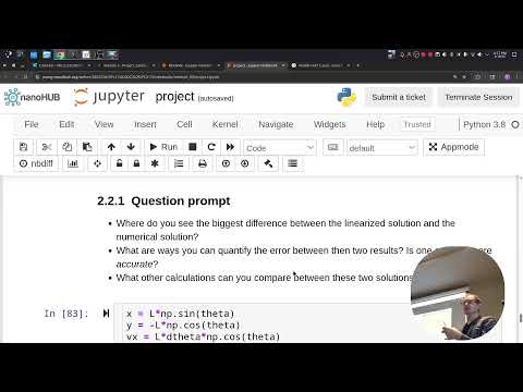
- After brief classroom logistics, Cooper resumes the pendulum analysis with a 90-degree initial angle.
- The next step is to use the already determined angular motion to calculate other engineering quantities.
- Cooper places the coordinate origin at the hinge and converts the pendulum’s fixed length and angle into x and y position.
- Because zero angle is defined as vertical, the coordinate relationships use sine and cosine differently than the standard polar convention.
- Differentiating position gives Cartesian velocity components, including the angular-rate term because theta varies with time.
- A quiver plot displays velocity vectors at positions along the pendulum’s path.
- The velocity vectors grow as the mass descends toward the bottom of the swing and shrink as it rises.
- Skipping vectors, such as plotting every fifth one, reduces clutter; equal axis scaling preserves the path’s shape.
- The radial force balance relates cable tension to gravity and centripetal acceleration, using the previously calculated angle and angular velocity.
- Cooper illustrates a 1-pound mass, converts pounds mass to slugs by dividing by 32.2, and uses feet-based units to obtain force consistently.
- The resulting tension over time can inform cable thickness and support-system design.
- Cooper compares linear and nonlinear tension curves and asks which model should guide a cable design.
- Designing for the higher predicted load is safer, while averaging the curves is less conservative; the nonlinear model may reduce material, cost, and weight.
- A bungee-swing failure example illustrates the danger of underestimating dynamic loads, especially near the bottom of a 90-degree swing where speed is highest.
- Kinetic energy follows from the tangential speed, giving a dependence on mass, pendulum length, and angular velocity squared.
- With zero potential energy at the bottom of the swing, the rise in height is L times one minus cosine theta, so gravitational potential energy is mgL(1 − cos theta).
- For an ideal pendulum with gravity and tension but no drag or friction, total kinetic plus potential energy should remain constant.
- At a 90-degree start, the linear model predicts more kinetic energy than the initial potential-energy change, while the nonlinear model’s energy curves agree more closely.
- Cooper reports nonlinear total energy near 5.79 foot-pounds with about 0.05 foot-pound variation, compared with a linear result around 6.4 ± 0.6 foot-pounds.
- Reducing the initial angle to 10 degrees makes the motion solutions align more closely, but a measurable energy discrepancy remains.
- The nonlinear pendulum’s restoring acceleration depends on sine theta, while the small-angle model replaces sine theta with theta.
- That linearized equation behaves like a spring system, whose potential energy is quadratic, 1/2 kx².
- The actual gravitational potential is cosine-based, so the linear model’s parabolic energy approximation explains the repeating difference between the energy curves.
- Cooper recommends identifying which curves differ, where the difference occurs, and which measurable quantity is being compared.
- For a 60-degree example, the linear period is about 2.7 seconds and the nonlinear period about 2.9 seconds, a difference of 0.1 seconds.
- Frequency comparisons can be made by taking the inverse of each period.
- The class plan includes independent reading on Monday, case problem four on Wednesday, independent work Friday the 17th, and a wrap-up on Monday the 20th.
- Cooper recommends using a notebook’s print preview to collect code and graphs, then saving the page as a PDF with Control-P or Apple-P.
- Project three is complete, and the course moves on to module four.
Transcript excerpt
0:19 Okay. All right, I sent it another money request and if that one doesn't get approved, I'm going to just, you know, I don't care enough, dude. Oh my god. I'm Which one are you fighting for? Any factor? mitosis mitosis mitosis mitosis mitosis is this? All right, you're real weird on that. That's what you said. No, I said mitosis. And then you said mitosis. mitosis Yeah, this one you don't need. First five minutes only write a paragraph in the little box. A week or less. A week or less. I saw it in the rubric on the other case studies with these
1:06 long things in the classroom right there. Is it like an ending? I'm sure all of them are ending. That's awesome. Are they an ending or are they a beginning? >> [groaning] >> Here we go. Now we're caught up. Okay, cool. We said it was a farm. It's a farm. Sounds ominous. Okay, cool. We're back. We let I think this one I think I'm showing like a curve with 90° initial angle, like amplitude 90. Yeah. Let's get the mic up.
1:54 There we go. Cool. So we have we have all this information about like what is what is the pendulum, where is it, how fast is it moving, how fast is it accelerating. The last last part is figuring out what can we do with that information. Like what what other things could we compare? So what else what else would we want to know about like a moving pendulum in this case?
2:45 Is angle the only thing that we care about ever? We could convert it to regular velocity. Yeah. How would you What would be like regular velocity? Like how fast this thing is moving? What do we want to call like
This is the start of the transcript. Save this video free for the whole transcript, searchable and time-coded.
In this course
Related notes
Summary, takeaways, and chapters were generated by AI from the video's transcript and may contain errors. The video belongs to its creator, Professor Ryan C. Cooper.