ME2120 - 001
Overview
Ryan C. Cooper extends a computational model of orbital motion by tracking both radius and angle, then converting polar coordinates into x-y paths. Using an Earth-centered example with a radius of about 42 million meters and a circular speed near 3,000 m/s, he compares circular, elliptical, and hyperbolic trajectories, and explains how simulation verification differs from experimental validation.
Key takeaways
- A radial solution does not uniquely determine an orbital path: both r(t) and θ(t) are needed to reconstruct x-y position.
- For a circular orbit at a radius near 42 million meters, a speed around 3,000 m/s yields a period on the order of 80,000 to 90,000 seconds.
- Changing only the initial speed produces distinct trajectory types: the baseline speed gives a circle, 1.2 times that speed gives an ellipse, and 1.5 times gives an unbound hyperbolic path.
- An escaping hyperbolic trajectory can have an angle that approaches a finite asymptotic value, rather than increasing through repeated full revolutions.
- Simulation verification checks whether the equations reproduce an expected result, such as constant radius for a circular orbit; validation requires comparison with experimental measurements.
- The same orbital equations can be reused for multiple initial conditions by placing the calculations in a loop and plotting each resulting trajectory.
Chapters
- The earlier calculation produced radius and radial-rate values over time, but a constant radius alone does not reveal the object's path.
- The example places the object about 42 million meters from Earth's center, with Earth modeled at roughly 6 million meters in radius.
- A circular orbit can have zero radial acceleration while still having nonzero total acceleration from gravity.
- The path requires both radius r(t) and angle θ(t), with x and y obtained from the polar-to-Cartesian transformation.
- Cooper uses the second equation of motion to calculate angular velocity, then cumulatively sums angular changes over time steps.
- For the circular-orbit case, the computed angle advances by roughly half a radian over the initial 10,000 seconds.
- At the baseline speed of about 3,000 m/s, the radius remains constant and the plotted x-y trajectory forms a circle.
- The orbit period is estimated from circumference divided by speed, using T = 2πr/v.
- With r near 42 million meters and v near 3,000 m/s, the period is on the order of 80,000 to 90,000 seconds.
- At 1.5 times the circular speed, approximately 4,600 m/s in the example, the radius grows as the object escapes rather than returning to orbit.
- The escape trajectory approaches a straight-line asymptote, and its angular coordinate tends toward a finite value near 2 radians.
- At 1.2 times the circular speed, the radius reaches maxima and minima and the x-y path develops into an ellipse.
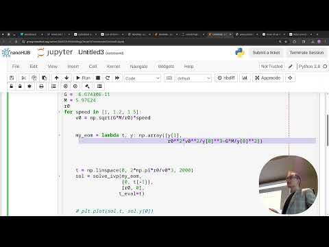
- Cooper wraps the repeated calculations in a loop so the circular, elliptical, and hyperbolic trajectories can be plotted together.
- The comparison plot labels all three paths and adds a blue point at (0, 0) to mark Earth.
- The same equations and computational steps apply across the cases; only the initial speed changes.
- The orbital angle is measured from the chosen x-axis, while the radius extends from Earth's center; the asymptote and radial angle become closer as distance increases.
- Polar or cylindrical coordinates simplify motion with circular structure, although setting up rotating reference frames requires extra work.
- The circular-orbit result is verified by agreement between the expected constant radius and the simulation; validation would compare a model against measured satellite motion.
- The next class project uses pendulum experiments to compare measured motion with linear and nonlinear models, while the case-problem work is due Tuesday.
Transcript excerpt
1:03 All right. I'm just trying to get back into where we left off last time. Woo. This [clears throat] week has been crazy. Just meetings and all sorts of stuff. Good Friday. It is a good Friday. Yeah. >> [laughter] >> The good Friday. Launch. All right. As that's loading up. All right. Last time we figured out how
1:51 fast this thing, at least the equation for like how fast this thing is moving, the debris, if it's going around in a circular orbit, so constant altitude. It's moving around. Um So, the next step is like if I know So, now we have r of t. It's going to be like And we even have like r dot of t. I've got like a whole kind of matrix
2:42 full of all these radii, all these radial change, like radius changes, like drdts. How do I go from that radius to like actually looking at what the path of this orbit looks like? Um I think last time we left off, we got Um probably untitled three. I should title
3:34 my notebooks, but So, this thing is up at and it'll catch up in a second, but 4.2 mil or 4.2 or 42 million meters, something like that. 1 2 3 4 5 6. Yeah, so 42 million meters from the center of the earth. And the earth is 6 million meters radius. Um all big numbers. That's the main thing with space. Everything's just like huge. Um except for a gravitational constant, which is super tiny. Negative 11, 10 to the negative 11. And then it's moving 3,000 m per second,
4:22 so 3 km per second. Um So, this is the radius over like 1,000. I think I create like 1,000 seconds or 10,000 seconds. It's just constant. It's not changing at
This is the start of the transcript. Save this video free for the whole transcript, searchable and time-coded.
In this course
Related notes
Summary, takeaways, and chapters were generated by AI from the video's transcript and may contain errors. The video belongs to its creator, Professor Ryan C. Cooper.