ME2120-002
Overview
Ryan C. Cooper reviews the final ME2120 project schedule, then compares analytical and numerical models of a pendulum to show when the small-angle approximation is useful. Using Python to solve the nonlinear equation of motion, the class examines amplitude, period, and phase, finding that 30° is a practical engineering cutoff and that a 180° initial position exposes a major difference between the linear and nonlinear models.
Key takeaways
- For a pendulum, the nonlinear equation uses angular acceleration −(g/L) sin(θ); the small-angle linearization replaces sin(θ) with θ.
- At a 30° amplitude, the linear and nonlinear pendulum periods are both approximately 2.7 seconds, with a plotted difference too small for the class’s roughly 0.05-second timing resolution.
- A 15° amplitude produces no measurable curve difference in the demonstrated plots, while 30° serves as Cooper’s practical engineering cutoff for a small angle.
- Amplitude can be measured from an oscillation graph as (maximum − minimum)/2, including when the equilibrium position is offset from zero.
- Matching initial position and velocity makes the analytical and numerical solutions start in phase; different periods can still cause their peaks to drift apart later.
- At exactly 180°, the nonlinear fixed-length model can remain balanced with zero angular acceleration, while the linear cosine model still predicts oscillation, illustrating the linear approximation’s limited range.
Chapters
- Project three is scheduled for the current class and Friday, followed by Monday for the reading assignment and case problem four starting Wednesday the 15th.
- Project four will follow case problem four; module four applies impulse, momentum, and energy methods that have already been introduced.
- Project five asks each group to apply one useful course concept to a career, hobby, or personal interest, using formats such as a report, PowerPoint, Jupyter notebook, or even an interpretive dance.
- There is no final exam or late penalty; groups can communicate whether they need until the last class day or the following Friday to finish project five.
- The pendulum exercise moves from a linear prediction and measured period to a comparison between analytical and nonlinear numerical solutions.
- Cooper uses a 5-foot-9-inch pendulum length and gravitational acceleration of 32.2 ft/s² to match Monday’s measurements.
- The analytical model predicts continued oscillation between +60° and −60° without decreasing amplitude.
- Damping would make the model more realistic, but requires measuring damping and changes the period only slightly for this exercise.
- The nonlinear angular acceleration is modeled as −(g/L) sin(θ), where g is gravity and L is pendulum length.
- The second-order equation is rewritten as two first-order equations: angular position changes at the rate of angular velocity, and angular velocity changes at the rate of acceleration.
- A Python initial-value solver advances the state over time and returns numerical values, allowing the same approach to handle linear or nonlinear systems.
- The numerical method is presented as a guided overview; students are not expected to build or edit the solver themselves.
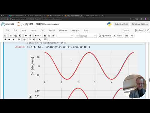
- The plots compare analytical predictions in blue with numerical predictions in red for angle, angular velocity, and angular acceleration.
- Students identify differences in amplitude, period, and apparent alignment between the two solutions.
- The class notes that pendulum length and gravitational acceleration affect the period, so comparisons depend on using consistent parameters.
- The initial 60° condition produces more visible disagreement than the later small-angle tests.
- Period is read as the time between repeated peaks; differentiating position to obtain velocity or acceleration does not change the oscillation period.
- For the large-angle comparison, the analytical and numerical periods appear separated by roughly 0.2 to 0.3 seconds on the plotted curves.
- Amplitude is calculated as half the difference between the maximum and minimum values, which works even when oscillation is centered around a nonzero equilibrium.
- The angle curves share a 60° amplitude, while velocity and acceleration curves have different amplitudes because they represent different physical quantities.
- Both models begin with the same initial position and angular speed, so their phase difference is zero at time zero.
- Different periods cause the curves to drift relative to one another, but the numerical period does not progressively change over time in the extended plot.
- The class estimates an approximately 2.7-second cycle for the plotted motion and checks whether the peak spacing changes across a longer time interval.
- Amplitude, frequency, and period provide clearer comparison measures than loosely describing the curves as simply out of phase.
- The central question is how small the initial angle must be for the linear and nonlinear solutions to become effectively indistinguishable.
- At 30° amplitude, the plotted acceleration curves show the largest visible difference, estimated as less than about 1%.
- The periods are both roughly 2.7 seconds, with plotted estimates near 2.77 and 2.74 seconds.
- Because classroom timing resolution was about 0.05 seconds, the period difference at 30° is not practically measurable with the available method.
- The class also tests a 15° amplitude and sees no measurable difference between the linear and nonlinear curves on the graphs.
- Cooper’s rule of thumb is to treat angles below 30° as small for typical engineering and physics calculations.
- A stricter 15° cutoff is also reasonable when greater accuracy is needed, but a usable threshold must be chosen for applying a linear model.
- The comparison emphasizes that calculated values can differ even when the difference is too small to measure or matter for the intended use.
- Students predict what happens when the pendulum starts at 180°, where the linear and nonlinear models behave very differently.
- The linear model continues to predict cosine-like oscillation because it assumes linear restoring behavior at every starting angle.
- In the nonlinear model, a perfectly balanced pendulum at 180° can remain stationary because the modeled angular acceleration is zero.
- The model assumes a fixed pendulum length, so falling or changing length is outside the problem’s stated constraints.
Transcript excerpt
0:00 It's crazy to talk to you. Are you guys allowed to Okay, we're back. Good. All right, it's loud. Feels loud. Loud is fine. So, logistic-wise, we have We just have a few weeks left in the semester. We're going to do Yeah. You should be proud of getting done. We're getting close. We are working on project three today and Friday. Monday,
0:49 we'll take a day off. Just take some time to like do the reading assignment. Then on Wednesday, the 15th, we'll be back, start working on Keep going to the wrong computer. Start working on like case problem four, spend a couple of days on that, and then then we'll spend two days on project four, like Mon- Monday, Wednesday, maybe we'll do like Wednesday, Friday on project four, like get through module four. Typically, so we're not ramping like nothing's ramping up. I know we're like turning in more assignments right now, but the difficulty is not. Like module four is typically the one that most people have the easiest time with looking at like impulse, momentum, and energy methods. Well, we've talked a lot about
1:38 that already, and we're just kind of applying it. And most of you have come out of thermodynamics recently, so like the idea of conservation of energy, we don't have to start from a square one. It's like already an idea that sort of things in. But this is the plan. Get through project three today, Friday. Take Monday off. Wednesday come back. Do case problem four for Wednesday, Friday, maybe Monday. And then project four. Then Then we'll get into the last week of class where we can the this module five project. I think I assigned everyone back into their project one groups. Uh but we can check on that. And
This is the start of the transcript. Save this video free for the whole transcript, searchable and time-coded.
In this course
Related notes
Summary, takeaways, and chapters were generated by AI from the video's transcript and may contain errors. The video belongs to its creator, Professor Ryan C. Cooper.