ME2120 - 001
Overview
Ryan C. Cooper derives the pendulum equation of motion using radial and tangential coordinates, then contrasts the exact nonlinear equation, θ̈ = -(g/L)sinθ, with its small-angle linearization, θ̈ = -(g/L)θ. He connects the linear model to natural frequency and period, predicts a 5 ft 9 in pendulum’s period, and compares that prediction with a classroom measurement to discuss error, model validation, and verification.
Key takeaways
- A pendulum with fixed length L has one degree of freedom, and its tangential force balance produces the exact equation θ̈ = -(g/L)sinθ.
- For small angular displacements measured in radians, replacing sinθ with θ yields a linear harmonic-oscillator model with angular frequency ωₙ = √(g/L).
- For a 5 ft 9 in pendulum with g = 32.2 ft/s², the linear model predicts a period of about 2.66 seconds, or a frequency of about 0.376 Hz.
- Timing 10 cycles reduces the relative effect of stopwatch reaction time compared with timing one cycle; the classroom result of about 27 seconds implies a period near 2.7 seconds.
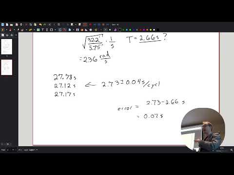
- The measured period differed from the prediction by approximately 0.07 seconds per cycle, illustrating that model comparison requires attention to both measurement uncertainty and the choice of reference value.
- Validation compares a model’s prediction with observed pendulum behavior, while verification checks whether different solution methods, such as linear and nonlinear approaches, give consistent results.
Chapters
- Ryan C. Cooper introduces the pendulum as Project 3, focusing on forming an equation of motion.
- The project compares a small-angle linearized equation with a numerical solution of the exact nonlinear equation.
- Cooper explains that rotational motion often produces nonlinear equations involving sine and cosine, which generally lack a simple handwritten solution.
- Because the bob moves along a circular arc, Cooper uses radial and tangential directions rather than Cartesian axes.
- Tension acts inward along the radius, while gravity is split into radial and tangential components using cosine and sine of θ.
- The free-body-diagram method follows the same sequence used in earlier course problems: identify forces, resolve components, and relate them to acceleration.
- The pendulum’s radius is its fixed length L, so ṙ = 0 and r̈ = 0.
- The angle θ is the system’s single degree of freedom, so one independent equation of motion is sufficient.
- The tangential equation gives θ̈ = -(g/L)sinθ, while the radial equation can later be used to find tension from the motion.
- For small angles in radians, sinθ is approximated by θ using the first term of its Taylor series.
- The nonlinear equation becomes θ̈ ≈ -(g/L)θ, a linear differential equation that is easier to solve and analyze.
- Cooper frames the approximation as useful in engineering because linear models support prediction and analysis even when the underlying system is nonlinear.
- The linearized pendulum behaves like a harmonic oscillator: greater angular displacement produces greater restoring acceleration.
- Its angular natural frequency is ωₙ = √(g/L), measured in radians per second.
- A full cycle corresponds to 2π radians, so frequency in hertz is f = ωₙ/(2π), and the period is T = 1/f.
- Cooper works through a pendulum length of 5 ft 9 in, converted to 5.75 ft, using g = 32.2 ft/s².
- The angular frequency is approximately √(32.2/5.75) = 2.36 rad/s, corresponding to about 0.376 cycles per second.
- Taking the inverse of the frequency gives a predicted period of approximately 2.66 seconds per cycle.
- The calculation highlights the need to use consistent units, including converting inches to feet when using gravity in ft/s².
- Cooper recommends timing 10 cycles rather than a single swing to reduce the effect of stopwatch start-and-stop reaction time.
- Measuring more cycles improves the average period estimate, though timing 100 cycles would take roughly 266 seconds based on the 2.66-second prediction.
- The class counts each full return to the starting position as one cycle and uses stopwatches to record the total time.
- The class records several times for 10 pendulum cycles, with reported totals clustered around 27.1 to 27.8 seconds.
- Dividing the elapsed time by 10 gives a measured period of roughly 2.7 seconds per cycle.
- The measured value is close to the 2.66-second prediction, with an approximate difference of 0.07 seconds per cycle.
- Cooper defines absolute error as the difference between predicted and measured values, giving about 0.07 seconds per cycle in this comparison.
- He distinguishes measurement uncertainty from the question of which value represents the system’s best estimate of the true period.
- For a pendulum’s natural frequency, Cooper leans toward using measured evidence as the baseline while recognizing that measurements are error-prone and physical models are useful.
- Cooper says the project will use Python to predict pendulum motion and compare the result with measurements.
- Agreement between prediction and measurement within an acceptable error, such as roughly 0.07 seconds per cycle, can support model validation.
- Verification is a separate check: compare linear and nonlinear solution approaches to see whether solving the problem in two ways produces consistent results.
- The next class is scheduled to examine verification and the comparison between linear and nonlinear models.
Transcript excerpt
0:10 This is how you Okay, welcome back.
1:07 We're going in coming in hot to the end of the semester. So, we have project three and then we'll do um one more case problem. Also, a little like case problem three was a little shorter than our first two. Kind of running out of time a little bit, but I think it was a nice exercise in like working in cylindrical coordinates and thinking about how things move, those kind of forces. We're going we'll wrap up. This is our uh pendulum project for project three. So looking at when we create an equation of motion uh if there's rotation in the in your motion usually you end up with like nonlinear equations because signs and cosiness end up having lots of answers
1:57 like infinite number of answers. It doesn't mean that they're impossible to solve. just means that there's no like handwritten solution. You can't just say like here's here's my function of time bless you. So that's what we're working on with this project is jumping into that. Sound good? All right. So there are two equations of motion that we're considering for a pendulum. Um a linearized solution and then this numeric then we'll look at a numerical solution of the exact differential equation. Do you know where these equation have you seen these before? Um got to get my mouse back.
2:47 Does this look familiar like from intro to physics or anything? Do you know where it comes from? Are they both true? Like it's first equation and second equation. Are they saying the same thing? Like they're both a pendulum. >> Yeah. >> The first one it's like only holds true for small values. >> Okay. >> For small values of theta. Um, yeah, that's true.
This is the start of the transcript. Save this video free for the whole transcript, searchable and time-coded.
In this course
Related notes
Summary, takeaways, and chapters were generated by AI from the video's transcript and may contain errors. The video belongs to its creator, Professor Ryan C. Cooper.