ME2120-002
Overview
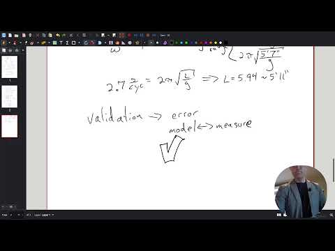
Ryan Cooper uses a pendulum project to connect free-body diagrams and cylindrical-coordinate dynamics with linearized predictions, frequency calculations, and experimental validation. For a 5 ft 9 in pendulum, the small-angle model predicts a natural frequency of about 2.36 rad/s, or 0.376 cycles/s, and a period near 2.65 s; classroom measurements give about 2.7 s, prompting discussion of measurement error, uncertainty, and acceptable model tolerance.
Key takeaways
- For a fixed-length pendulum, the tangential force balance gives θ̈ = -(g/L) sin θ, while the radial balance is used to calculate string tension.
- The small-angle approximation sin θ ≈ θ turns the nonlinear pendulum equation into simple harmonic motion with natural angular frequency √(g/L).
- For a 5 ft 9 in pendulum under g = 32.2 ft/s², the linear model predicts about 2.36 rad/s, 0.376 Hz, and a 2.65 s period.
- Timing 5 cycles in about 13.4 s and 10 cycles in about 27.1 s yields measurements near 2.7 s, illustrating why multi-cycle timing reduces reaction-time effects.
- The predicted-to-measured difference is about 0.05 s, or roughly 1.9 percent; whether that is acceptable depends on measurement uncertainty and engineering tolerance.
- Uncertainty in pendulum length propagates into the period prediction through T = 2π√(L/g), so validation should account for input uncertainty as well as stopwatch error.
Chapters
- Ryan Cooper introduces Project 3 after wrapping up motion predictions for circular, elliptical, and escape trajectories in Case Problem 3.
- The pendulum project compares linearized and numerical solutions with a measured motion.
- The governing pendulum equation includes sin θ, while the familiar simplified form uses the approximation sin θ ≈ θ.
- A central project question is how small the angle must be for the approximation to remain sufficiently accurate.
- Cooper chooses cylindrical coordinates because the bob moves along an arc, avoiding more cumbersome Cartesian-component algebra.
- The string tension acts radially toward the pivot; gravity has both radial and tangential components.
- With a fixed pendulum length L, radial velocity and acceleration terms involving changes in radius are zero.
- The tangential force balance produces the equation of motion, a second-order differential equation in θ.
- The radial balance instead determines the constraint force, tension, once θ and its angular velocity are known.
- The nonlinear equation is θ̈ = -(g/L) sin θ; its structure follows from gravity acting along the pendulum's path.
- Replacing sin θ with θ yields θ̈ + (g/L)θ = 0, the linear simple-harmonic-oscillator equation.
- The linearized model has an exact time-dependent solution, making it possible to predict the pendulum's position at any future time.
- Large rotations generally create geometric nonlinearities, while linear approximations are useful over a limited range of motion.
- The small-angle natural angular frequency is ωₙ = √(g/L), measured in radians per second.
- Ordinary frequency is f = ωₙ/(2π) in cycles per second, and the period is T = 1/f = 2π/ωₙ.
- One complete oscillation corresponds to 2π radians; a half-cycle carries the pendulum from one side to the other.
- In the ideal model, no damping force is included, so the oscillation does not lose energy or amplitude.
- Using L = 5.75 ft and g = 32.2 ft/s² gives ωₙ ≈ 2.36 rad/s.
- The corresponding frequency is about 0.376 cycles/s, or 0.38 Hz, and the predicted period is approximately 2.65 s.
- Cooper emphasizes that frequency and period are practical quantities to measure, including at high rates with sensors and frequency analysis.
- The class measures elapsed time over several oscillations rather than timing a single cycle.
- Recorded results include about 13.4 s for 5 cycles and 27.1 s for 10 cycles, giving periods around 2.7 s.
- Timing several cycles and averaging helps reduce the impact of reaction time and stopwatch uncertainty.
- Comparing the measured period of about 2.70 s with the predicted 2.65 s gives an absolute difference of about 0.05 s.
- Relative error is about 0.05/2.70, or 1.9 percent, depending on which value is treated as the best estimate.
- Cooper contrasts a rationalist preference for the calculated model value with an empiricist emphasis on the measured result.
- An uncertainty of roughly ±2 in in the pendulum length changes the predicted period range because T = 2π√(L/g).
- Whether a 0.05 s discrepancy is acceptable depends on the application's tolerance and the reliability of the timing method.
- A model is validated when its predictions agree with measurements within the required tolerance; Cooper previews comparing linear and nonlinear solutions next.
Transcript excerpt
0:00 Breaking news. >> That sounds like better news than normal news. >> I don't know. Breaking news usually indicates something very terrible has happened >> or something very terrible. >> Well, I remember breaking news. I'm pretty sure it's like there's like some teachers in high school. I I said the wrong unit. >> Oh my god. >> No, I don't know. >> Tell us. How did I an analogy? >> No. No. Personal experience. How dare you? >> Okay.
0:53 Welcome back. >> We are working on [laughter] >> What are you trying to say? [clears throat] >> I'm trying to say. Okay, we are working on module three for uh for we kind of wrapped up the case problem three last week. Um thanks for being here and if you couldn't make it totally fine like it was good Friday and Easter weekend but um there we did some nice work of like predicting motion for case problem three to wrap that up. Main thing is like look like going through the
1:42 equations of motion for that case problem and then looking at the different paths of motion for those three different cases like circular orbit elliptical and then the one that sort of flies off into space like loses. Um, so now we're on to project three where we're looking at a pendulum and we've got we're going at this from every angle. We're going to beat this horse to death of like every type of every type of answer to a pendulum equation. Um, we have a linearized solution, we have a numerical solution, and then today we'll even have >> a measured value of like what is the motion of a pendulum? like how do we how
2:30 do we measure it and what are the things
This is the start of the transcript. Save this video free for the whole transcript, searchable and time-coded.
In this course
Related notes
Summary, takeaways, and chapters were generated by AI from the video's transcript and may contain errors. The video belongs to its creator, Professor Ryan C. Cooper.