ME2120 - 001
Overview
Professor Ryan C. Cooper outlines the remaining ME2120 assignments, then uses a Python pendulum simulation to compare a linearized small-angle model with the exact nonlinear equation of motion. The class examines a 5-foot pendulum, tests initial angles from 10° to 180°, and finds that 30° is a practical small-angle rule of thumb, while large angles reveal meaningful differences in period and acceleration.
Key takeaways
- An ideal pendulum simulation without damping should preserve amplitude because tension does no work and gravity conserves mechanical energy.
- A second-order pendulum equation can be solved numerically by expressing it as two first-order equations for angle and angular velocity, then passing the system to a Python initial-value solver.
- The small-angle approximation sin(θ) ≈ θ is visually excellent at 10° and remains practically useful around 30°; near 40°, period differences in the example remain within roughly ±0.05 seconds of measurement uncertainty.
- The linearized model predicts acceleration proportional to angle without bound, whereas the exact nonlinear model's angular acceleration is bounded by g/L for a fixed pendulum.
- A pendulum released exactly at 180° with zero speed remains at rest in the ideal nonlinear model because the gravitational torque is zero, although the equilibrium is physically unstable to small disturbances.
- For a large release angle such as 160°, the exact nonlinear pendulum takes longer to complete its motion, and its angular and centripetal acceleration peaks occur at different points in the swing.
Chapters
- Project Three on pendulum motion is due Friday, followed by Module Four reading and Case Problem Four work.
- Project Five is a group reflection on applying dynamics to a career, hobby, or other interest, not a cumulative report.
- Project Five rough drafts can be brief notes; final submissions may use PowerPoint, a report, a Jupyter notebook, or another format.
- There is no final exam or late penalty, and students may submit Project Five during finals week after providing a plan during the last week of class.
- Cooper sets up a 5-foot pendulum swinging between 60° and -60° and compares its simulated motion with a measured period.
- The ideal model includes gravity and string tension, with tension doing no work and gravity acting as a conservative force.
- Because the model includes no damping or other energy loss, the pendulum's amplitude should not decrease over time.
- The second-order pendulum differential equation is rewritten as two first-order equations for angle and angular velocity.
- The state vector stores the current angle and angular rate; the equations return angular rate and angular acceleration.
- Python's numerical solver advances the initial-value problem in time, producing a table of values rather than a closed-form function.
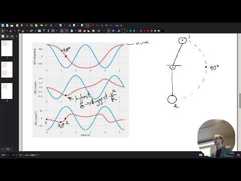
- The simulation plots angle, angular velocity, and angular acceleration for the linearized and nonlinear models.
- The two angle curves begin at the same initial condition, but their peaks drift apart as their periods differ.
- Amplitude is read from the vertical range of a graph, while period is measured between repeating points such as consecutive peaks.
- The exact angular acceleration depends on sin(θ), so its magnitude is bounded by g/L for a fixed pendulum length.
- The linearized model uses θ in place of sin(θ), making its predicted acceleration grow without bound as the angle increases.
- At a 60° initial angle, the nonlinear model can therefore show lower angular velocity and acceleration amplitudes than the linear model.
- Students vary the initial angle and speed to investigate when sin(θ) is close enough to θ for the linear model.
- Changing pendulum length or gravity should affect the period according to the previously derived dependence on the square root of L/g.
- The key test is whether differences between the linear and nonlinear curves are large enough to matter for the intended measurement.
- At an initial angle of 10°, the linear and nonlinear position curves nearly overlap, making their difference difficult to see on the plot.
- At 40° to 41°, position and velocity remain fairly close, and the period difference is within the class's approximate measurement uncertainty of ±0.05 seconds.
- Cooper recommends 30° as a convenient rule of thumb for using the small-angle approximation, while noting that longer observations can reveal model differences.
- At exactly 180° with zero initial angular velocity, the nonlinear model has zero gravitational torque and remains stationary under its ideal assumptions.
- The linearized equation does not represent the inverted equilibrium accurately and predicts a large acceleration instead.
- The model constrains the pendulum to a constant-radius circular path, so it does not simply fall straight down or allow the string length to shrink.
- At 160°, the nonlinear pendulum starts near the inverted position and accelerates increasingly as it falls toward the bottom.
- The nonlinear period grows as the initial angle becomes large, while the linearized model does not capture that amplitude-dependent change.
- Angular acceleration is greatest around 90°, while centripetal acceleration is greatest at the bottom, where angular speed is highest.
- The project prompt asks students to compare linear and nonlinear results by quantifying differences in amplitude, frequency, and phase.
- The curves share their initial conditions and therefore start in phase, even though their later motion can diverge.
- Cooper plans to explore additional pendulum calculations and plots on Friday to finish Project Three.
Transcript excerpt
0:43 It's quiet. We ready though. Okay. So, plan kind of coming into last couple of weeks. Um on Friday, we're going to wrap up module three and turn in this project. We're working on pendulum looking at on Monday we Monday. Yeah, Monday we looked at actual pendulum measured time period which we can turn into frequency and natural frequency like radians per second and all that. Um and then on Yeah. So turn that in Friday. Monday we'll um we'll take the day off like no class spend some time finishing
1:32 up the the reading assignment for module 4 so that Wednesday Friday we can work on case problem four um wrap it up Monday and then we'll get two more days for project four and that'll be the end the end of all of my like assigned things. Then we'll take couple of class periods to uh apply some like come back to our project one proposals where we were thinking about like how does how do how does dynamics get applied to different careers, hobbies and those kind of things. That's the plan. questions, concerns,
2:21 affirmations, like we can do it. Yeah, it's getting close. Um, we're not I'm not trying to like ramp up anything like we're not we're not getting into like harder material or anything. So, as long as we're just consistently like putting in some time to the class, I don't foresee like anyone like, "Oh my god, there's so many extra assignments right now." Like, we're it's the same cadence that we've been doing. A little bit faster, but not like we're not doing anything like harder than than what you've already done. So, I'm trying to plan out. My main goal is not to like add extra big projects as finals and
This is the start of the transcript. Save this video free for the whole transcript, searchable and time-coded.
In this course
Related notes
Summary, takeaways, and chapters were generated by AI from the video's transcript and may contain errors. The video belongs to its creator, Professor Ryan C. Cooper.