ME2120-002
Overview
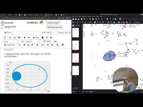
Ryan C. Cooper uses Python to numerically solve the radial and angular equations for an object orbiting Earth, then compares circular, elliptical, escape, and collision trajectories as initial speed changes. The class also distinguishes numerical verification, checking a solution against expected behavior, from validation, comparing a model with experimental measurements planned for a pendulum.
Key takeaways
- The orbit model separates radial motion from angular motion: solve r(t) numerically, then use theta dot = r0 v0 / r(t)^2 to recover angular position.
- At the modeled radius of about 42 million meters, the circular-orbit simulation remains constant to within a few millimeters over 250,000 seconds.
- Changing initial speed changes orbit type: the class demonstrates a circle at the reference speed, an ellipse at 1.2 times that speed, and an escape trajectory at 1.5 times that speed.
- An object slower than circular speed can still remain on an ellipse; an impact occurs only when the trajectory's closest approach intersects Earth's physical radius.
- Explicit integration can introduce visible numerical wiggles, while an implicit integration method reduces them in the demonstrated orbit simulation.
- Verification and validation answer different questions: verification checks whether numerical results match expected behavior, while validation checks whether predictions match experimental measurements.
Chapters
- Cooper frames the work as combining kinematics, how an object moves, with kinetics, why it moves.
- The model has two degrees of freedom: orbital radius r and angle theta.
- A Python initial-value solver will compute radius and radial velocity over time, avoiding a focus on analytical differential-equation methods.
- After solving for r(t), the class uses the angular-rate relation theta dot = r0 v0 / r(t)^2 to find angular motion.
- For the circular-orbit case, radius stays near 42 million meters, with numerical variation of only a few millimeters over 250,000 seconds.
- The angular-rate plot is essentially flat, and converting radius and angle to x and y produces a circular path around Earth at the origin.
- Increasing initial speed to 1.5 times the circular-orbit value makes radius grow instead of remaining constant.
- As the object moves far from Earth, the gravitational term becomes negligible and the angular position approaches a horizontal asymptote.
- The x-y plot shows a flyby or escape trajectory rather than a closed orbit; the example speed is about 4.6 kilometers per second.
- At 1.2 times the circular speed, radius first increases and then decreases, demonstrating an oscillating radial distance.
- The angle continues to increase, while angular speed varies as radius changes through the orbit.
- The plotted path is an ellipse with Earth at one focus, not at its center, and the class compares it with the circular and escape paths.
- Cooper plots Earth at its actual size and lowers the initial speed to test whether the trajectory intersects the planet.
- A speed below the circular-orbit value does not automatically mean an immediate impact: the object can remain on an ellipse until its closest approach falls within Earth.
- Explicit numerical integration produces small wiggles; an implicit method reduces them, while conserved angular momentum helps explain why the ideal trajectory does not simply spiral inward.
- The class reduces speed further and identifies a path that would hit Earth or pass through the atmosphere.
- Students are asked to turn in their differential-equation work and graphs; Cooper plans to post the Python code on HuskyCT.
- The next project begins with pendulum experiments, and students are asked to consider how pendulum motion can be measured.
- Verification checks whether the numerical model reproduces an expected result, such as a circular orbit at roughly 42 million meters with millimeter-scale error.
- Validation compares model predictions with measurements, a process planned for the pendulum work.
Transcript excerpt
0:00 Who cares? I set my timer for 30. >> I set for I set mine for 35 and I show you. >> Well, you can set set your time for your wash. >> My phone timer. >> You don't use your phone. >> Are you one of those people who just the laundry? >> No, no, no. I I I just like look at I look at the clock. Oh, yeah. >> And I'm usually right in like 500. >> Dude, I one time I one time took this. So, I sorted my laundry and this [clears throat] guy had his laundry in uh the dryer for an hour. >> Um no, no. So I finished washing my stuff and what's it called? Um I finished washing my stuff like when I got there. >> Ready? >> No.
0:49 >> Where's Luke? >> I think >> we did we did most of the hard work Monday and Wednesday. At this point, we're just trying to like post-process all of our work of like once you identify um how the thing moves, your kinematics, why the thing moves, your kinetics, and then put those two together. Um in this case, I'm using Python to actually get me answers for like how big is the radius, how far is this thing moving? But you can use any kind of method. Um yeah, we were just talking about like lelass transforms. There's probably a le applause transform for this kind of equation where you have like an R dot 1 over R2 and an R in
1:39 there or a V^2 over R. Yeah, like a V ^2 over R, an R 2 and R cubed. I think there is a lelastrant you would end up with um oh my god I can't remember but anyway I'm sure there is
This is the start of the transcript. Save this video free for the whole transcript, searchable and time-coded.
In this course
Related notes
Summary, takeaways, and chapters were generated by AI from the video's transcript and may contain errors. The video belongs to its creator, Professor Ryan C. Cooper.