Math 1153 - 9 November 2026 - Chapter 14
Overview
Mike Jacobsen introduces Chapter 14 confidence intervals for a population mean, μ, using the sample mean, sample standard deviation, and a t critical value. He demonstrates the inverse-t calculator process and works through a pickpocket-loss example, finding a 95% interval of $405.08 to $621.56, then begins a dementia-age example that requires calculating summary statistics from raw data.
Key takeaways
- For a confidence interval estimating a population mean, use y-bar ± t-star × s/√n, with degrees of freedom n − 1.
- The inverse-t calculator input for a two-sided confidence interval is the left-tail area (1 − C)/2 and df = n − 1; report the positive magnitude of the resulting left-tail value.
- Quantitative data call for the parameter μ and statistics y-bar and s, while categorical data call for p and p-hat.
- For 25 pickpocket offenses with mean loss $513.32 and standard deviation $262.23, a 95% interval is $405.08 to $621.56 and the margin of error is $108.24.
- When only raw quantitative observations are supplied, calculate y-bar and s with one-variable statistics before finding the standard error or confidence interval.
- A practical interpretation must state the confidence level, what population mean is being estimated, the relevant population, and both interval endpoints.
Chapters
- Exam 3 is scheduled for Monday before Thanksgiving break and covers Chapters 6 and 7 through Section 13.3.
- Bring a calculator and prepare one page of notes, front and back.
- Jacobsen recommends finishing quizzes and MyLab first, each worth 15% of the course grade, then practicing with the two sample exams.
- A confidence interval for a population mean has the form y-bar ± t-star times SE(y-bar).
- The standard error is s divided by the square root of n, and the interval estimates μ.
- Unlike the Chapter 13 proportion interval, this method uses the sample standard deviation and a t critical value rather than z-star.
- For a two-sided confidence interval, calculate the left-tail area as (1 − confidence level) / 2.
- Use the calculator's inverse-t function with that area and degrees of freedom, df = n − 1.
- For 99% confidence and n = 190, use area 0.005 and df 189; inverse t returns a negative left-tail value, so report the positive critical value 2.6021.
- At 99% confidence, the example's t critical value is 2.6021, slightly larger than the z critical value 2.58.
- The t distribution accounts for estimating the population standard deviation σ with the sample standard deviation s.
- The t and normal critical values become more similar as sample sizes grow, but t-star remains the appropriate value when σ is estimated.
- The first application uses an FBI crime-data context and a simple random sample of 25 pickpocket offenses.
- The sample mean loss is $513.32, and the sample standard deviation is $262.23.
- Because losses are numerical dollar amounts and the prompt gives a sample mean, the data are quantitative and the target parameter is μ, not a population proportion p.
- Define μ as the population mean loss in dollars for all pickpocket offenses in the specified area.
- A complete parameter statement identifies both the measured variable, dollar loss per offense, and the population, all offenses in that area.
- For quantitative data, use μ and y-bar with s; for categorical data, use p and p-hat.
- The standard error of the sample mean is SE(y-bar) = s / √n.
- Substituting s = 262.23 and n = 25 gives SE(y-bar) = 52.4460 dollars.
- Jacobsen recommends retaining four decimal places during intermediate calculations to reduce rounding error.
- For 95% confidence, the left-tail area is (1 − 0.95) / 2 = 0.025.
- With n = 25, degrees of freedom are 24; the calculator's inverse-t routine gives t-star = 2.0639.
- On a TI calculator, open the distribution menu with second and bars, choose inverse t, and enter the area and df.
- Substitute y-bar = $513.32, t-star = 2.0639, and SE = $52.4460 into y-bar ± t-star × SE.
- The resulting interval is approximately $405.08 to $621.56, rounded to the nearest cent.
- The interval estimates the population mean loss μ, rather than the loss in any single pickpocket offense.
- A context-based interpretation says there is 95% confidence that the mean loss for all pickpocket offenses in the area lies between $405.08 and $621.56.
- The margin of error is t-star × SE(y-bar), which is $108.24 for this example.
- The margin of error shows why reporting only the sample mean of $513.32 would conceal substantial uncertainty.
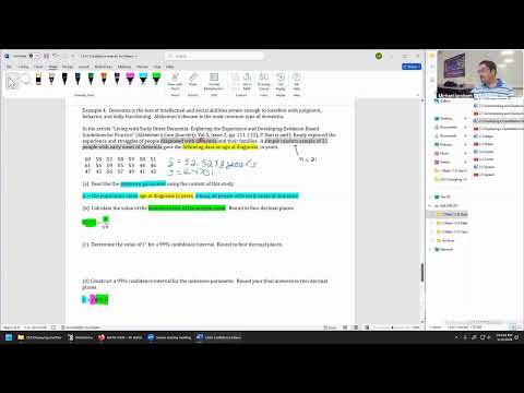
- The second application uses ages at diagnosis, in years, from a simple random sample of 21 people with early-onset dementia.
- Because the problem supplies raw quantitative observations rather than y-bar and s, enter the values in calculator list L1 and run one-variable statistics.
- The sample statistics are y-bar = 52.5238 years and s = 6.4701 years.
- Define μ as the population mean age at diagnosis, measured in years, among people with early-onset dementia.
- Jacobsen notes that the population wording may need to specify people diagnosed with the condition if diagnosis status differs from having the condition.
- The standard error is 6.4701 / √21 = 1.4119 years.
- The dementia example has y-bar = 52.5238, s = 6.4701, n = 21, and SE = 1.4119; the target interval is at 99% confidence.
- The next calculation requires df = 20 and the 99% left-tail area of 0.005 to find t-star with inverse t.
- Jacobsen postpones the remaining t-star and interval calculations until the next class after the writing pad fails.
Transcript excerpt
0:53 Well, I think we can start. Welcome back, everyone. The big announcement for the day is absolutely that we have our third exam coming up. This one's going to be on Monday of next week, right before going on to the Thanksgiving break, covering sections, well, chapters starting chapter 6, chapter 7 up to these sections ending on 13.3. 13.3 is where we did a confidence interval procedure. And so that's pretty much going to be the roundup for this third exam. The content we're working on is similar. It's still a confidence interval, but that's for quantitative data. So, now is a good time to start working on putting together your page of notes. Just like on the other exams, it'll be two, one page front and back. Be sure to bring your calculator as
1:40 well. And for studying, a good order of operations to be prepared for this exam is absolutely make sure you're fully caught up on all the quizzes. That's a great start. That's 15% of the grade and so it has some of the fastest return on a points versus time basis. After that, getting caught up on my lab helps out as well. That's also worth 15% of the grade. The questions are pretty similar. And once you get fully caught up for the work on my lab according to this material here, then that'd be a good time to start looking into the sample exams, two versions just like on the other exams. But any questions at the moment folks with the upcoming exam. Okay. Well, let's get started then.
2:36 We're in chapter 14. There's a lot of concepts that goes together in chapter 14. So, we did a lot of their really hard conceptual work when we right before going on to the weekend last
This is the start of the transcript. Save this video free for the whole transcript, searchable and time-coded.
In this course
Related notes
Summary, takeaways, and chapters were generated by AI from the video's transcript and may contain errors. The video belongs to its creator, Mike Jacobsen.