Math 1153 - 27 October 2026 - Section 13.1
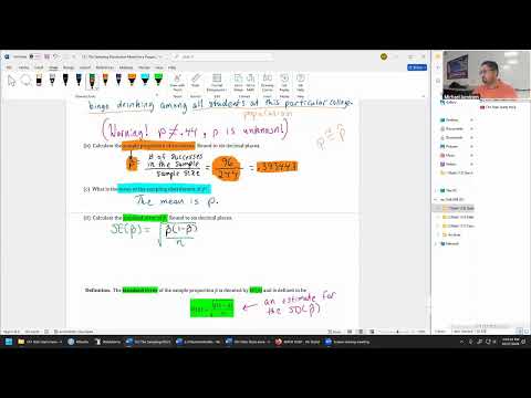 Watch on YouTube →
Overview
Mike Jacobsen introduces sampling distributions for sample proportions and explains the proportion version of the central limit theorem: the sampling distribution of p̂ is centered at p, has standard deviation √[p(1−p)/n], and becomes approximately normal when the sample size is adequate. Using RStudio simulations and examples about workplace social-network etiquette and binge drinking at one college, he distinguishes the unknown population proportion from the sample statistic and shows how to estimate the standard deviation with the standard error.
Key takeaways
- For a sample proportion p̂ from a population with success rate p and sample size n, the sampling distribution has mean p and standard deviation √[p(1−p)/n].
- Approximate normality depends on both sample size and the population proportion: p = 0.56 works well at n = 50 in the simulation, while p = 0.93 requires a larger sample, with n = 200 looking nearly normal.
- A contextual definition of p must specify the success and the population; the 44% national binge-drinking rate cannot be treated as the unknown rate for students at one particular college.
- When p is unknown, estimate the sampling distribution's standard deviation with SE(p̂) = √[p̂(1−p̂)/n], using the observed sample proportion.
- In the college example, 96 binge-drinking admissions among 244 students produce p̂ = 0.393443 and an estimated standard error of 0.031274.
Chapters
- Mike Jacobsen defines a success or failure outcome for a single categorical variable and uses p̂ = successes/n to estimate population proportion p.
- In the workplace-etiquette example, 56% of surveyed social-network users said it was not okay to friend their boss, so p̂ = 0.56.
- Quiz 8 on linear regression is due Thursday; Wednesday office hours are canceled because of a mandatory department meeting.
- Jacobsen imagines repeatedly sampling 50 social-network users and calculating a new p̂ for each sample.
- A single study might produce p̂ = 0.56, while another sample could produce a different value, such as 0.565.
- Collecting many repeated values of p̂ and plotting them reveals the sampling distribution for sample size n = 50.
- The classroom demonstration assumes the true population proportion is p = 0.56 and the sample size is 50.
- RStudio simulates 1,000,000 samples and plots the resulting sample proportions in a histogram.
- The sampling distribution represents the possible values of p̂ across samples of the specified size, not the distribution of individual survey responses.
- With p = 0.56 and n = 50, the simulated histogram is roughly symmetric and bell-shaped, with its peak near 0.56.
- Values far from 0.56, such as around 0.30, are possible but occur very rarely in the million simulated samples.
- Jacobsen distinguishes the population of social-network users from the separate population of possible sample-statistic values.
- Changing the assumed population proportion to p = 0.93 changes the shape of the sampling distribution.
- At n = 5, simulated sample proportions are strongly left-skewed, so a normal model is unsuitable.
- Comparisons with n = 10, 25, and 50 show that increasing sample size reduces the skew.
- For p = 0.93, the histograms at n = 100 and n = 150 look progressively more symmetric, although some left skew remains visible.
- At n = 200, the sampling distribution appears very close to normal and is centered near 0.93.
- Proportions close to zero or one generally require larger samples for an approximately normal sampling distribution.
- For a random sample of size n from a population with success proportion p, the sampling distribution of p̂ has mean p.
- Its standard deviation is √[p(1−p)/n], also written √(pq/n) when q = 1−p.
- When n is sufficiently large and p is not too close to zero or one, the distribution of p̂ is approximately normal.
- The example assumes a study of 100 social-network users, with the reported sample proportion p̂ = 0.56.
- Jacobsen defines p in context as the population proportion of all social-network users who say it is not okay to friend their boss.
- He explains that a contextual parameter definition must identify both the success and the full population, which also helps make later conclusions precise.
- For a hypothetical calculation, the example assumes p = 0.53 and n = 100, even though the true population proportion is generally unknown.
- Substituting into √[p(1−p)/n] gives √[0.53 × 0.47 / 100], or approximately 0.0499.
- Jacobsen demonstrates entering the expression into a calculator either as one parenthesized expression or through successive operations using the previous answer.
- Because the standard deviation formula depends on unknown p, it cannot generally be calculated exactly from a real sample.
- The standard error substitutes the observed sample proportion p̂ for p: SE(p̂) = √[p̂(1−p̂)/n].
- This plug-in estimate supports later confidence intervals and margin-of-error calculations while acknowledging that p remains unknown.
- A university administrator samples 244 students at one college; 96 say they engaged in binge drinking during the past week.
- The stated national rate of 44% concerns college students nationwide, not the population at the administrator's particular college.
- The relevant p is the proportion of all students at that college who admitted to binge drinking, and it is unknown.
- The sample proportion is 96/244 = 0.393443 when rounded to six decimal places; it must remain a proportion, not be converted to 39.3443% in the formula.
- The central limit theorem says the mean of the sampling distribution of p̂ is p, the unknown proportion at this specific college.
- Using 0.44 as that mean would be incorrect because 44% is a national result, not a measured rate for the sampled college.
- Substitute p̂ = 0.393443 and n = 244 into SE(p̂) = √[p̂(1−p̂)/n].
- The estimated standard deviation of the sampling distribution is approximately 0.031274, rounded to six decimal places.
- Jacobsen shows calculator shortcuts for reusing the stored answer when entering p̂ twice in the standard-error expression.
- The main ideas covered include defining p in context, calculating p̂, applying the central limit theorem, and computing standard error.
- Jacobsen says students can begin the Section 13.1 MyLab homework with these tools and notes that the class will revisit the material Thursday.
- The lecture ends before completing every remaining item in the section, with a plan to continue in the next class.
Transcript excerpt
0:52 Well, it's time. Welcome back everyone. We are just starting out in chapter 13. We took a look at some of the bigger ideas in that chapter. Some of the notation for the new parameter, the new statistic dealing with proportions. So, we're going to take another really careful look at sampling distributions, see what's going on in this chapter, and possibly move on into the next section rather. But aside from that, not a whole lot of announcements today. The quiz number eight on linear regression is going to be due on Thursday. But I did have one unfortunate thing that came up with the office hours. I haven't had this happen so far this semester. So, this always kind of sucks when it happens. But I do have a mandatory department meeting that I have to join on Wednesday, tomorrow, which is overlapping with the office hours,
1:39 unfortunately. I can reschedule for anyone that want to meet on that Wednesday tomorrow. And I don't expect to have any other cancellations like this one that should occur at any other point of the semester. This looks like it's kind of a one-time thing. So, sorry if you're intending to come to that office hours. I'll send out an announcement as a reminder. And if you want to connect and want to find a different time, don't hesitate to reach out. But any questions or comments at all, folks, before we start off today. Okay, let's get started. So, we're now really just getting started in section
2:28 13.1 just on the very first example. And well, there's lots of scribbling there. This is about where we left off. Let's kind of refresh slowly. Let me see if I can zoom in to hide some of that stuff. We're looking into specifically
This is the start of the transcript. Save this video free for the whole transcript, searchable and time-coded.
Related notes
Summary, takeaways, and chapters were generated by AI from the video's transcript and may contain errors. The video belongs to its creator, Mike Jacobsen.