Math 1153 - 17 November 2026 - Sections 15.1, 15.3
Overview
Mike Jacobsen shows how to formulate and carry out a one-proportion hypothesis test, moving from defining the population parameter and hypotheses to calculating a test statistic, p-value, and contextual conclusion. In the student-attendance example, a 2000 sample of 8,302 students had a 33% no-absence rate versus the 1996 benchmark of 34%; the test gives z = -1.9234 and p = 0.0272, which is significant at α = 0.05 but not at α = 0.01.
Key takeaways
- For categorical data with success and failure outcomes, define P as the population success proportion; the sample proportion p̂ is a statistic and does not appear in the hypotheses.
- A question about whether a proportion has declined from a benchmark becomes a left-tailed test: H₀: P = P₀ and Hₐ: P < P₀.
- In a one-proportion hypothesis test, assume H₀ is true and calculate the test standard deviation with P₀: √[P₀(1 − P₀)/n].
- For the attendance sample, p̂ = 0.33, P₀ = 0.34, and n = 8,302 produce z ≈ −1.9234 and a left-tail p-value of approximately 0.0272.
- The attendance result is significant at α = 0.05 because 0.0272 < 0.05, but it is not significant at α = 0.01 because 0.0272 ≥ 0.01.
- A hypothesis test can support or fail to find evidence for the alternative, but it cannot establish that the null hypothesis is true; define the hypotheses and α before collecting data.
Chapters
- The previous example compared gold-card customers’ mean tenure with the 17.3-month mean for regular-card customers.
- Because the question asks whether tenure is the same or different, the alternative is two-tailed: μ ≠ 17.3.
- The null represents no population difference, while the alternative captures the company’s research question.
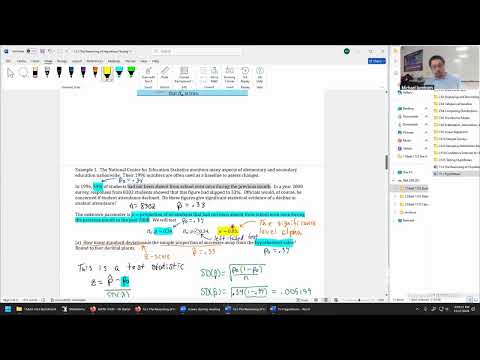
- The education example defines success as a student not being absent even once during the previous 30 days.
- The data are categorical because each student falls into one of two outcomes: no absence or at least one absence.
- For categorical success/failure data, the parameter is a population proportion, P.
- In 1996, 34% of students had no absences during the previous month, providing the hypothesized population proportion, P₀ = 0.34.
- The 2000 survey included 8,302 students and reported a sample proportion of 0.33, written as p̂ = 0.33.
- The sample statistic p̂ is not part of the hypotheses; the hypotheses describe population parameters.
- The parameter is P, the proportion of all elementary and secondary students nationwide in 2000 who had no absences during the previous 30 days.
- The problem compares the 2000 population with the 1996 benchmark, so the year and student population belong in the parameter definition.
- The question asks about a decline, establishing a directional, left-tailed alternative.
- The null hypothesis states no change from the 1996 benchmark: H₀: P = 0.34.
- The decline question becomes Hₐ: P < 0.34, with the alternative expressing the research claim.
- The 33% sample result is evidence to evaluate, not a value to place in either hypothesis.
- For a sample proportion p̂, the central limit theorem gives an approximately normal sampling distribution when success-failure conditions are met.
- The sampling distribution has mean P and standard deviation √[P(1 − P)/n].
- The test compares the observed p̂ with the hypothesized population proportion under the null.
- The first testing assumption is that H₀ is true, so P is treated as the specified null value P₀.
- With P₀ known, the test’s standard deviation is calculated using √[P₀(1 − P₀)/n].
- The test statistic measures how many standard deviations the sample proportion lies from P₀.
- The significance level α is the required evidence threshold for rejecting H₀.
- If the p-value is strictly less than α, reject H₀ and report significant evidence for Hₐ.
- If the p-value is greater than or equal to α, fail to reject H₀; do not claim that the null has been proven true.
- The worked test uses H₀: P = 0.34, Hₐ: P < 0.34, p̂ = 0.33, n = 8,302, and α = 0.05.
- The prompt’s wording, asking how many standard deviations p̂ is from the hypothesized value, calls for the test statistic z.
- For hypothesis testing, use P₀ in the standard deviation formula because the null is assumed true.
- The null-based standard deviation is √[0.34(1 − 0.34)/8,302], approximately 0.0052.
- Substituting the sample proportion gives z = (0.33 − 0.34)/0.0052 ≈ −1.9234.
- The negative z-score reflects that the observed no-absence rate is below the 34% benchmark.
- The p-value is the standard normal area at z = −1.9234 and farther into the left tail, matching Hₐ: P < 0.34.
- On a TI calculator, use normalcdf with a lower bound of −10^99, upper bound −1.9234, mean 0, and standard deviation 1.
- The resulting p-value is approximately 0.0272.
- Because 0.0272 < α = 0.05, reject H₀.
- The contextual conclusion is that the study found significant statistical evidence that the 2000 population proportion with no absences was below 34%.
- A hypothesis-test conclusion addresses the direction in Hₐ; estimating the size of the change would require a confidence interval.
- Changing α does not change the observed test statistic or p-value; it changes only the decision threshold.
- At α = 0.01, 0.0272 ≥ 0.01, so the decision is to fail to reject H₀.
- The contextual conclusion must then say the study failed to find significant evidence of a decline; the setup also must be fixed before data collection rather than adjusted afterward.
Transcript excerpt
0:54 Well, welcome back everyone. Looks like we can get started. So, we're on week number 13 and this is one of the harder weeks to attend. Not just because it's a busy week with the exam three that we're getting through, but also we're right before the break. But we'll still have class today. We'll still have class on Thursday. I appreciate you all making it in on one of the harder weeks to attend. And if you were watching this later, you didn't make it this week, that's okay, too. You'll be here in spirit if you watch this lecture, get through the homework problem at some point, homework problems, rather with where we're at today. We're going to finish off the last example in section 15.1. The whole purpose of 15.1 is to show us how to set up the hypothesis in hypothesis testing the null and alternative hypothesis.
1:43 Then the next section we're going to look at the full procedure. The reading is involving two sections but 15.2 was such a short one I couldn't see any good exercises to really assign. It's just rolled into 15.3 as well. So we're going to do 15.3 as a complete section including the 15.2 two and see what the full hypothesis test looks like from the very start as we did it in 15.1 to the very end making conclusions. So that's where we're at so far. But any questions or comments at all folks to start us out today. Okay, let's jump back in. Here's the
2:31 problem that we were looking at before going on to the weekend. The instructions on this was to define the unknown parameter and then state the null hypothesis, this one, and an alternative hypothesis, just one of them. We have to pick the right one, in
This is the start of the transcript. Save this video free for the whole transcript, searchable and time-coded.
In this course
Related notes
Summary, takeaways, and chapters were generated by AI from the video's transcript and may contain errors. The video belongs to its creator, Mike Jacobsen.