Math 1153 - 22 October 2026 - Chapters 7, 10
 Watch on YouTube →
Overview
Mike Jacobsen finishes a Chapter 7 regression example by calculating a residual, interpreting the slope and y-intercept, and explaining why predicting a Wright meter reading from a Mini-Wright value of 250 is unsafe extrapolation. He then introduces Chapter 10 inferential statistics, distinguishing populations, samples, parameters, and statistics, and demonstrates how Excel can select a simple random sample to estimate a population mean while emphasizing that estimates need a margin of error.
Key takeaways
- For participant five, the observed Wright meter value of 476 minus the predicted value of 495.95 gives a residual of −19.95, so the regression model overpredicted that reading.
- The regression slope is interpreted as a change in the predicted Wright meter reading for each one-unit increase in the Mini-Wright reading, with the y-variable’s units in the numerator.
- A y-intercept is meaningful only if x = 0 is plausible in the study context; a zero Mini-Wright reading is not a reasonable ordinary lung-strength measurement.
- A Mini-Wright input of 250 is far below the study’s observed minimum of 346, so using the fitted line there is extreme extrapolation rather than a dependable prediction.
- A convenience sample of six students from one Math 1153P class cannot represent all Fall 2026 ISU students, regardless of whether the sample is enlarged.
- A simple random sample gives every possible sample of the same size an equal selection chance, but even a representative sample needs a margin of error to communicate uncertainty.
Chapters
- Mike Jacobsen expects to grade the second exam on Friday and upload marked exams, including students’ notes pages, to Canvas.
- Quiz 7 is due, and Quiz 8 is posted; Jacobsen says Quiz 8 resembles the current regression example.
- He resumes the paired-measurement example involving 10 participants measured with a portable Mini-Wright meter and a larger Wright meter.
- Each participant has paired values from both devices, so the Mini-Wright reading is the explanatory variable and the Wright meter reading is the response.
- The scatter plot shows a reasonably strong linear relationship, supporting a least-squares regression model.
- Entering a Mini-Wright reading of 500 into the fitted equation predicts a Wright meter reading of 495.95.
- A residual is observed response minus predicted response, written as e = y − ŷ.
- For participant five, the observed Wright meter value is 476, while the model predicts 495.95 for the Mini-Wright value of 500.
- The residual is 476 − 495.95 = −19.95, indicating that the prediction was higher than the observed reading.
- Jacobsen’s slope-interpretation template identifies the x-variable, y-variable, direction of change, and slope magnitude.
- The horizontal axis represents Mini-Wright readings and the vertical axis represents Wright meter readings, so slope units are Wright meter units per Mini-Wright unit.
- The positive slope is about 0.75, meaning the predicted Wright meter reading increases by about 0.75 units for each one-unit increase in the Mini-Wright reading.
- The y-intercept describes the model’s predicted response when the explanatory variable x equals zero.
- Here, x = 0 would mean a person’s Mini-Wright reading is zero, which is not a plausible ordinary measurement for a living, breathing participant.
- Jacobsen contrasts this with a prior algae-and-grazers example, where zero grazers was meaningful and the intercept could be interpreted in context.
- The smallest Mini-Wright observation in the study is 346, making an input of 250 far outside the observed data range.
- Using the regression line at 250 is extreme extrapolation, so the prediction should not be trusted without additional data.
- The relationship might change outside the measured range, for example by becoming nonlinear; Jacobsen notes that measurements from children could follow a different pattern.
- Jacobsen shifts from Chapter 7 to Chapter 10, introducing inferential statistics as the next major course topic.
- A population is the complete collection of individuals or objects of interest; the example population is all ISU students registered for Fall 2026.
- A sample is the subset selected for study, while a parameter describes a population and a statistic describes a sample.
- The population parameter μ is the mean GPA of all ISU students registered for Fall 2026.
- The sample statistic is the sample mean GPA, denoted ȳ in the course’s textbook, calculated from six students in the Math 1153P section 30 class.
- Students from one online class are not representative of all ISU students, so their sample mean cannot validly estimate the population mean.
- Selecting classmates because they are readily available creates a convenience sample, which may systematically omit students from other courses or in-person programs.
- A biased, nonrepresentative sample makes the statistic a poor approximation of the population parameter, even if the sample size is increased.
- A simple random sample of size n gives every possible sample of that size an equal chance of selection, helping produce a representative sample.
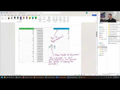
- Jacobsen builds a demonstration population of 20 students and selects a sample of six.
- Excel’s RAND() function assigns each student a random number between 0 and 1; copying and pasting the values freezes the lottery numbers.
- Sorting by random number and taking the six largest selects the sample, illustrating how random selection avoids choosing only convenient participants.
- Once the sample is representative, its mean GPA, ȳ, can be used as an estimate of the unknown population mean μ.
- Inferential statistics uses a sample statistic to draw conclusions about an underlying population parameter.
- The Excel selection is a classroom demonstration of random sampling, not a required quiz or homework procedure.
- A random, representative sample addresses sampling bias but does not eliminate uncertainty in the estimate.
- Jacobsen says an estimate remains incomplete unless its error, often described by a margin of error, is quantified.
- Confidence intervals and hypothesis tests will provide tools for describing uncertainty in later inferential-statistics work.
- A prior ceramic hip-replacement example estimated a population proportion using p̂ = 6.99%; like a mean estimate, it still required a margin of error.
- Quantitative data use parameters such as μ and sample means such as ȳ, while categorical data use population proportions and statistics such as p̂.
- Jacobsen previews further work on conclusions permitted by different data types and by observational studies versus experiments, then pauses the lesson until Monday.
Transcript excerpt
0:54 and it's official. We're on our Thursday class to close out week number nine. Welcome back everyone and congratulations on getting through the second exam if you've already completed it. I'll begin grading this exam on Friday. And because this is my first class I have that I gave an exam out, I'll be working on our class first. So, I have a pretty decent chance of getting this one done on Friday. Not so much on my other classes that I gave an exam this week. But you should expect to see this graded on Friday. And once it's complete, I'll be uploading your marked upgraded exam, including your page of notes as the last two pages on the exam as well up here in grade. that you'll be able to find in Canvas. But aside from that, with what we've got going on today, the rest of the week is just an ordinary week. Our quiz 7 is due
1:43 and our quiz number eight is now posted. Quiz 8 is pretty similar to the questions we're working on, in particular, example number two. And quiz 7, you can look into the section or chapter six, and there's plenty of questions inside there that are very similar to that question as well. But any questions or comments at all to start us out today. Okay. Well, let's begin. We only just started example two. So now we're going to come back in finish this example. It was dealing with two measurements of
2:32 looking into measures of lung strength. Well, two instruments on making a medical measurement of lung strength. One was a smaller device called the mini rate meter and it made all of these measurements here on 10 participants. This one is easy to transport. You can put in your back pocket. But if you want
This is the start of the transcript. Save this video free for the whole transcript, searchable and time-coded.
Related notes
Summary, takeaways, and chapters were generated by AI from the video's transcript and may contain errors. The video belongs to its creator, Mike Jacobsen.