Math 1153 - 29 October 2026 - Sections 13.1, 13.2
 Watch on YouTube →
Overview
Mike Jacobsen connects the central limit theorem for sample proportions to margin-of-error estimation, using a survey of 244 students with 96 reported binge drinkers to illustrate a sample proportion of 0.393443 and an approximate 95% interval of 33.09% to 46.00%. He then explains the four conditions for using the normal model and applies them to a cancer-treatment sample, where only 8 of 25 patients survived at least five years, so the success-failure condition fails.
Key takeaways
- For the 244-student survey, p-hat = 96/244 = 0.393443 and the estimated standard error is 0.031274, producing an approximate 95% interval from 33.09% to 46.00%.
- Because the campus interval includes the 44% national rate, the survey does not provide statistically significant evidence that the campus binge-drinking proportion is lower.
- The estimated standard error for a sample proportion is √(p-hat(1-p-hat)/n), a plug-in estimate of the sampling distribution's standard deviation.
- Using a normal model for p-hat requires independence, randomization, a sample no larger than 10% of the population, and at least 10 observed successes and 10 failures.
- In the cancer-treatment example, 8 of 25 patients surviving at least five years fails the success-failure requirement, even though the sample was random and had 17 failures.
- A sample proportion and its margin of error must be considered together; the point estimate alone cannot establish a statistically significant difference.
Chapters
- Mike Jacobsen frames Section 13.1 as a transition from descriptive statistics, such as histograms and sample means, to inferential statistics.
- The central limit theorem describes the sampling distribution of statistics such as the sample proportion, p-hat.
- For a population proportion p and sample size n, the sampling distribution of p-hat has mean p and standard deviation √(p(1-p)/n).
- Because p is unknown, estimate the standard deviation with the standard error, substituting p-hat for p and 1-p-hat for 1-p.
- The sampling distribution becomes approximately normal when n is sufficiently large and p is not too close to 0 or 1.
- A random sample of 244 students included 96 who admitted to binge drinking, giving p-hat = 96/244 = 0.393443.
- The 44% national rate is a comparison benchmark, not the unknown campus population proportion p.
- A sample estimate alone cannot establish that the campus rate is below the national rate; its margin of error must also be considered.
- Substituting p-hat into the standard-deviation formula gives an estimated standard error of about 0.031274.
- The standard error describes the typical variation in sample proportions across repeated samples of 244 students from the same campus.
- Repeated samples would generally produce different p-hat values, even though they estimate the same underlying population proportion.
- Jacobsen adapts the 68-95-99.7 empirical rule to the sampling distribution, treating p as its center and the standard error as an estimate of its standard deviation.
- Approximately 95% of sample proportions fall within two standard errors of p under the normal-model conditions.
- For the campus example, the approximate margin of error is 2 × 0.031274, or 0.0625.
- The estimated interval is p-hat ± 2 standard errors: 0.393443 ± 2(0.031274).
- The resulting bounds are approximately 0.3309 and 0.4559, or 33.09% to 46.00%.
- The margin of error is about 6.25 percentage points, measured from the sample estimate to either endpoint.
- The 95% interval for the campus proportion includes the national benchmark of 44%, so the sample does not establish a statistically significant difference.
- An estimate near 39.3% cannot justify a claim that the campus rate is lower without accounting for the interval's upper bound.
- A hypothetical upper bound of 43% would exclude 44% and support evidence that the campus proportion is lower.
- Jacobsen introduces four requirements for applying the central limit theorem to sample proportions: independence, randomization, the 10% condition, and the success-failure condition.
- These conditions determine whether the sampling distribution of p-hat can reasonably be treated as approximately normal.
- The next examples focus on assessing the conditions before using normal-based margin-of-error methods.
- Responses may not be independent if students answer a sensitive binge-drinking question publicly and are influenced by earlier responses.
- Randomization requires a random or representative sample; selecting 244 students at a tailgate would risk selection bias.
- The 10% condition requires the sample to be no more than 10% of the population, so 244 students is reasonable for a large university but not a college of 500.
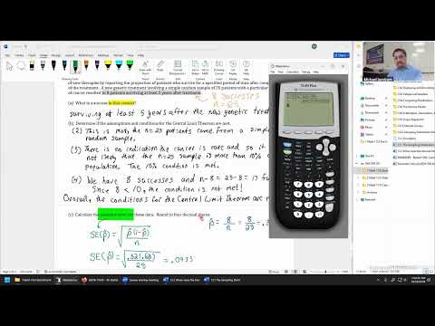
- The example describes a simple random sample of 25 patients with a particular cancer who received a new genetic treatment.
- Eight patients survived at least five years after treatment, making that outcome the success; the other 17 are failures.
- Defining success precisely is necessary to calculate p-hat and check the success-failure condition.
- The stated simple random sample of 25 patients satisfies the randomization condition.
- The problem gives no indication that the cancer is rare, so the sample is treated as unlikely to exceed 10% of the relevant population.
- A rare cancer with only about 100 patients would make a sample of 25 too large for the 10% condition.
- The success-failure condition requires at least 10 successes and 10 failures; this sample has 8 successes and 17 failures.
- Because 8 is below 10, the condition fails and the normal approximation for p-hat should not be used.
- A small success count can produce a skewed sampling distribution, requiring a different statistical method.
- The sample proportion is p-hat = 8/25 = 0.32, with q-hat = 0.68.
- The estimated standard error is √(0.32 × 0.68 / 25) = 0.0933, rounded to four decimal places.
- Although the standard-error calculation is straightforward, the failed success-failure condition means the normal-model inference is not appropriate; Section 13.3 will develop interval-based conclusions.
Transcript excerpt
1:05 Welcome back everyone. Looks like I kind of lost track of time. We've spent time to start up for about 10 seconds now, but welcome back. Happy Thursday. We're almost through the 10th week. And with what we have going on, we're just about to finish off section 13.1, move into the very next section. But not too much to say for the announcements. Any questions at all from you before we start out today? Okay, and welcome back. Sorry for zoning out for 10 seconds or so, but you know, as long as we start within the minute, I think we're doing pretty good. So, let's review back what we're doing in section 13.1.
1:51 This is some of the more abstract work that we'll do pretty much all semester. We're bridging the gap between descriptive statistics, just things like Y bar, the sample mean, plotting histograms, interpreting them them, those kinds of things, into the work on inferential statistics, when we're looking into the central limit theorem. So, let's take a look where we left off on our second example. We're down here, but just to kind of get caught up where we were for a good warm up. The major purpose for both examples two and three were all about the central limit theorem for proportions. The idea with this theorem says, when we go to measure a statistic, like the sample proportion P hat, or even the
2:41 sample mean Y bar, it comes from a new distribution. The central limit theorem says, the statistic P hat is the proportion successes in a random sample of size N, it'll come from a population which has true proportion of successes P. However, that value is going to be the unknown. That's what we're trying to estimate. The rules say, the mean of the sampling
This is the start of the transcript. Save this video free for the whole transcript, searchable and time-coded.
Related notes
Summary, takeaways, and chapters were generated by AI from the video's transcript and may contain errors. The video belongs to its creator, Mike Jacobsen.