Lecture 18 - An Aside on Errors & Uncertainties
Overview
Nathan Seifert explains how to report measurement uncertainty and propagate input errors through calculated outputs. The lecture distinguishes precision from accuracy, establishes two-significant-digit uncertainty reporting, and derives root-sum-of-squares propagation using partial derivatives, with examples including the ideal gas law and logarithmic and trigonometric functions.
Key takeaways
- A measurement reported with its mean and standard deviation communicates both its central value and spread; for a normal distribution, ±1 standard deviation covers about 68% of observations.
- Report uncertainties with two significant digits and round the measured value to the same decimal place; parenthetical notation such as 1.00120(32) m encodes an uncertainty of 3.2 × 10⁻⁴ m.
- For independent input uncertainties, propagate them with σᵧ = √Σ[(∂f/∂xᵢ)²σᵢ²], evaluating each derivative at the measured input values.
- For n = PV/RT with P = 1 bar, V = 2.10 L, and T = 298 K, the stated input uncertainties produce about 0.0848 mol with an uncertainty near 0.00098 mol.
- Addition and subtraction use quadrature of absolute uncertainties, while products and quotients use quadrature of fractional uncertainties to combine inputs with different units.
- Exact quantities such as mathematical coefficients and SI-defined constants contribute no uncertainty; the revised SI fixes constants including the speed of light and Avogadro’s constant.
Chapters
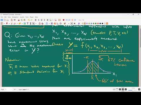
- Seifert frames experiments as apparatuses that take measured inputs such as pressure, temperature, and volume and produce an output such as heat capacity.
- The lecture addresses two tasks: reporting uncertainty clearly and calculating output uncertainty from uncertain inputs.
- Examples connect the method to lab measurements of molar mass and equilibrium constants.
- The notation x̄ᵢ denotes the mean of measurements of input xᵢ, while σᵢ denotes its standard deviation.
- A distribution of repeated temperature readings illustrates how measurements vary around their mean.
- A smaller standard deviation means a narrower spread and therefore greater precision.
- For a normal, symmetric measurement distribution, the interval from one standard deviation below to one above the mean contains about 68% of values.
- Accuracy concerns how close the mean is to the true value; precision concerns the spread of measurements.
- The mean and standard deviation provide a standardized way to communicate a measurement and its uncertainty.
- Seifert gives a measurement near 1.0012 m with an uncertainty of 3.2 × 10⁻⁴ m as a reporting example.
- The uncertainty should be reported with two significant digits, and the measured value should extend to the same decimal place as the uncertainty.
- The reporting convention is presented as a standard used broadly in chemistry, including by IUPAC.
- Rounding an uncertainty near 3 to one significant digit can represent a broad range, approximately 2.5 to 3.49.
- Reporting about 3.2 narrows the rounding range and communicates the uncertainty much more precisely.
- Two significant digits are a practical convention for keeping the rounded uncertainty itself reasonably well determined.
- In parenthetical notation, the digits in parentheses give the uncertainty in units of the final digits of the reported value.
- A value such as 1.00120(32) m means an uncertainty of 32 × 10⁻⁵ m, or 3.2 × 10⁻⁴ m.
- The alternative is explicit plus-or-minus notation, with both the value and uncertainty written before the unit.
- Defined mathematical quantities such as π and exact coefficients such as 3/2 do not contribute uncertainty to a calculation.
- For example, the 3/2 coefficient in the ideal-gas energy expression is exact, even when measured temperature is uncertain.
- Measured quantities still carry experimental uncertainty, so exact constants do not remove the need to propagate measurement errors.
- Seifert discusses the SI revision adopted in 2018 and implemented in 2019, which fixed selected fundamental constants at exact values.
- The speed of light is defined as exactly 299,792,458 m/s, and Planck’s constant as exactly 6.62607015 × 10⁻³⁴ J·s.
- The gas constant is exact in the revised system, so its uncertainty is not included when propagating experimental errors.
- Avogadro’s constant is fixed at exactly 6.02214076 × 10²³ entities per mole.
- The former mole definition linked the amount to 12 g of carbon-12, making the result dependent on precise mass measurement.
- The lecture contrasts that approach with the international prototype kilogram in Paris, whose mass drifted over time through contamination and other tiny physical changes.
- For an output y = f(x₁, …, xₙ), a partial derivative describes how sensitive y is to a small change in one input.
- The derivative is evaluated at the measured or mean input value, turning an input change into an estimated output change.
- For U = 3RT/2, temperature uncertainty maps to energy uncertainty through ∂U/∂T = 3R/2.
- Adding absolute error contributions directly gives a worst-case bound and can substantially overestimate typical uncertainty.
- A geometric right-triangle argument shows that independent contributions combine by the Pythagorean theorem rather than by a linear sum.
- For y = f(x₁, …, xₙ), the standard propagation formula is σᵧ = √Σ[(∂f/∂xᵢ)²σᵢ²], with derivatives evaluated at measured input values.
- For n = PV/RT, the inputs are pressure, volume, and temperature, while R is treated as exact.
- The partial derivatives are V/RT for pressure, P/RT for volume, and −PV/(RT²) for temperature.
- Using P = 1 bar, V = 2.10 L, T = 298 K, and uncertainties of 0.010 bar, 0.01 L, and 1 K gives n ≈ 0.0848 mol and σₙ ≈ 9.8 × 10⁻⁴ mol.
- The derivatives also make unit consistency checkable: each propagated term has units of moles squared before taking the square root.
- For sums and differences of quantities with matching units, combine absolute uncertainties in quadrature.
- For products and quotients, use fractional uncertainty, δx = σₓ/|x|, so errors in inputs with different units can be compared.
- For a product or quotient of independent inputs, the squared fractional uncertainty of the result is the sum of the squared fractional uncertainties of the inputs.
- For y = ln(x), derivative-based propagation gives σᵧ = σₓ/|x|.
- For y = sin(x), propagation gives σᵧ = |cos(x̄)|σₓ, with the cosine evaluated at the measured input.
- Seifert closes by emphasizing that derivatives act as sensitivity and unit-conversion factors between input changes and output changes.
Transcript excerpt
0:00 request and I think it's a good lecture to have. I think it went pretty well last month. I did it for the other section as well. Um I'm going to cut a few things that I told them for you guys to get through a little more information today. Um if you like I wanted if I was just going to say if there's like anything that you take from this class, this would be a really good lecture to take like your brain for the future. Um and that's the measurement and is we're going to talk about reporting error uncertainties and calculating them as well. Um we the first the first lab that guys for the people who are in the lab. Uh the first lab you did was steor lab you did these like errors and uncertainty calculations. There's like this worksheet. Um this is a a followup to that.
0:49 It's the same content but done not on piece of paper but now on a lecture form in some of the formulas that we used in that worksheet. Um basically what what I want to get out of here two things. One is if you have some measured value of some error or uncertainty how do you report it properly? That's one thing we're going to talk about. Second thing we're going to talk about is you have some measurements. You have let's say you you have some inputs to a experiment you know temperature pressure volume that have uncertainties then your experiment measuring as a function of those say I've got a box that measures entropy pressure and temperature um what's the error in entropy given the
1:38 error in the inputs. So that's a really nice thing to think about. You know, if you're measuring
This is the start of the transcript. Save this video free for the whole transcript, searchable and time-coded.
In this course
Related notes
Summary, takeaways, and chapters were generated by AI from the video's transcript and may contain errors. The video belongs to its creator, Nathan Seifert.