ENGR 201 Fall 2026 - Lecture 03: 2D Equilibrium of a Particle
Overview
Bruno Guidio introduces 2D particle equilibrium through the vector condition ΣF = 0 and the component equations ΣFx = 0 and ΣFy = 0. He demonstrates a four-step free-body-diagram method with three engineering examples: two cable-tension problems and a sailboat force-balance problem, emphasizing angle geometry, sign conventions, weight conversion, and solving two unknowns from two equations.
Key takeaways
- For a 2D particle in equilibrium, ΣFx = 0 and ΣFy = 0 provide two independent equations, so they can determine at most two unknown force magnitudes or directions.
- A reliable solution sequence is to draw a free-body diagram, resolve each force into signed x- and y-components, write both equilibrium equations, and solve the resulting system.
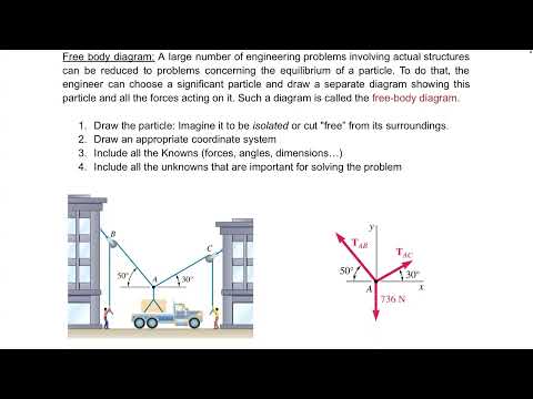
- For the 736 N box supported by cables at 30° and 50°, the equilibrium solution is approximately T_AB = 647.2 N and T_AC = 480.4 N.
- Mass must be converted to weight before using force equilibrium: a 6 kg load has weight 6 × 9.81 ≈ 58.86 N.
- A 3-4-5 triangle gives direction ratios directly, cos θ = 4/5 and sin θ = 3/5; those ratios are component multipliers, not angles to insert into a sine or cosine function.
- When an angle is measured from the y-axis, the x-component uses sine and the y-component uses cosine; component signs still depend on the force's actual direction.
Chapters
- Bruno Guidio asks students to record attendance using a QR code and opens class with a prayer.
- He notes that recording and screen-sharing are affected by Zoom and internet issues, and mentions a second statics section.
- Homework is due that night, and the lecture will continue the previous work on vectors and forces.
- A particle model ignores an object's size and shape, treating all applied forces as acting at one point.
- Guidio distinguishes particle problems from rigid-body problems, where size and shape matter.
- The class applies this idealization to engineering situations such as a box lifted by cables.
- A particle is in equilibrium when the vector sum of all applied forces is zero.
- In 2D, equilibrium requires ΣFx = 0 and ΣFy = 0, using the x- and y-components of each force.
- The two independent equations can solve up to two unknowns, such as force magnitudes or directions.
- A free-body diagram removes visual clutter and retains the particle, force vectors, relevant angles, and axes.
- Guidio's workflow is to draw the free-body diagram, resolve forces into components, apply equilibrium equations, and solve for unknowns.
- Cables are represented by tension forces, while a suspended box's weight acts downward.
- The first example asks for tensions in cables AB and AC supporting a box with a stated weight of 736 N.
- The free-body diagram places T_AB, T_AC, and the weight at point A, making the box a particle model.
- T_AC is resolved using a 30° angle, while T_AB uses a 50° angle; the downward weight contributes −736 N in y.
- The x-equilibrium equation is T_AC cos 30° − T_AB cos 50° = 0.
- The y-equilibrium equation is T_AC sin 30° + T_AB sin 50° − 736 = 0.
- Guidio substitutes one tension in terms of the other, warning students not to omit the sine factor when substituting into the y equation.
- Guidio asks students to show calculation steps because rounding intermediate trigonometric values can slightly change the result.
- He reminds students to set calculators to degrees, since the example uses 30° and 50°.
- The tensions are approximately T_AB = 647.2 N and T_AC = 480.4 N, with small differences possible from rounding.
- The second problem asks for T_AB and T_BC to support a 6 kg mass at point B.
- Guidio converts mass to weight with W = mg, using g = 9.81 m/s², giving approximately 58.86 N.
- The AB cable's direction comes from a 3-4-5 triangle, while BC is oriented at 45°.
- The AB direction can be represented by cos θ = 4/5 and sin θ = 3/5, or by calculating θ ≈ 36.87°.
- For the chosen axes, T_AB has components −(4/5)T_AB in x and +(3/5)T_AB in y.
- Students work through the component setup and compare the angle-based method with the fraction-based method.
- The x-equilibrium equation balances the leftward AB component against the rightward x-component of T_BC.
- The y-equilibrium equation combines the upward cable components and subtracts the 58.86 N weight.
- The calculated tensions are approximately T_AB = 42.0 N and T_BC = 47.6 N; Guidio clarifies that sine of 36.87° is not sine of 3/5.
- The third example gives a 40 lb force along AB and a 60 lb force along AE, and asks for the drag force F_D and tension T_AC.
- Guidio represents the sailboat forces as concurrent forces acting at point A.
- The diagram's dimensions are used to find the directions of the unknown cable and drag force before resolving components.
- For the first geometry, α = tan⁻¹(7/4) ≈ 60.26°.
- For the second geometry, β = tan⁻¹(1.5/4) ≈ 20.56°.
- The free-body diagram uses T_AC at β from the y-axis, the 40 lb force at α, F_D along positive x, and the 60 lb force downward.
- Because β is measured from the y-axis, T_AC contributes T_AC sin β in x and T_AC cos β in y.
- The 40 lb force points up and left, so its x-component is negative and its y-component is positive.
- F_D acts entirely along positive x, while the 60 lb force acts entirely downward along negative y.
- The y-equilibrium equation determines T_AC from T_AC cos 20.56° + 40 cos 60.26° − 60 = 0.
- Guidio obtains T_AC ≈ 42.89 lb, then substitutes it into the x-equilibrium equation.
- The resulting drag force is approximately F_D = 19.67 lb; the class closes with a reminder that Thursday's lecture will continue with more 2D equilibrium problems.
Transcript excerpt
0:11 All right. So, first of all, I will try the attendance uh code and this class. So please take a minute right now for you to scan the code. Write your last name and first name if you have done so. So every single time uh I'm with the code over there you can just come to the class and do it. All right. And then father, son, holy spirit. Amen. Director Lord, we beseech you our actions by holy inspirations and carry them on by grace's assistance that every prayer and work of ours may begin our ser and through you come to completion through Christ our Lord. Amen. Father,
1:00 Son, Holy Spirit. Amen. All right. So, you guys had a great holiday weekend. All good. Great. So, let's work now. Now the iPad is not going to work. I just screen share this one. See way internet is not helping me. Why is that? Because of Zoom. Let's see. Okay, got it. Record again. Share screen.
1:55 Okay, hopefully it's going to record. If not, I will just check it out and record to them in the next section. Okay, I didn't mention it, but I do have another section for statics. Okay. So, I'll try to figure it out here how to record and I will record one one lecture from here, one lecture from there. So, in case you're going to watch the lecture, it is not what I mention here exactly the same words is because I record the other section. Sounds good. Okay. Ready to waste a few minutes? Great. So, don't forget homework is due to tonight. Okay. If you have any questions, please come to me. Um but we're going to continue on our um work with vectors and force today. Okay. And today we're going to talk
This is the start of the transcript. Save this video free for the whole transcript, searchable and time-coded.
In this course
Related notes
Summary, takeaways, and chapters were generated by AI from the video's transcript and may contain errors. The video belongs to its creator, Bruno Guidio, PhD.