ENGR 201 Fall 2026 - Lecture 24 - Shear & Moment Diagrams (Graphical Method)
Overview
Bruno Guidio teaches the graphical method for constructing shear and bending-moment diagrams without repeatedly cutting a beam or deriving piecewise equations. He shows how point loads create shear jumps, distributed loads change shear gradually, and signed areas under the shear diagram give moment changes, using two beam examples to illustrate equilibrium checks, diagram shapes, and curve concavity.
Key takeaways
- A shear diagram can be built from left to right by adding upward forces and subtracting downward forces; concentrated loads cause vertical jumps, while a uniform distributed load causes a linear shear change.
- The shear diagram should return to zero at the beam end when the vertical reactions and applied loads satisfy equilibrium.
- The change in bending moment over an interval equals the signed area under the shear diagram, so moment values are found by accumulating areas from a known starting moment.
- Constant shear yields a straight-line moment segment, while linearly varying shear yields a parabolic moment segment whose concavity follows the direction of shear change.
- For the second example, the 3 kN/m load over 4 m has a 12 kN resultant for reaction calculations, but its distributed character must be represented as a gradual 12 kN decrease in shear.
- The first example's shear levels are −20, +26, and −14 kN, and its moment levels are −50 and +28 kN·m before returning to zero.
Chapters
- Bruno Guidio situates Lecture 24 within internal-force analysis of structures, following section cuts and piecewise shear and moment equations.
- The graphical approach uses load patterns and diagram geometry to analyze an entire beam without repeatedly writing equations in x.
- The lecture also notes that the section 3 final exam is scheduled for Tuesday at 1:00, with students asked to report three or more finals on the same day.
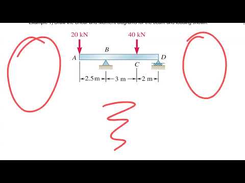
- For the first overhang-beam example, Guidio starts with support reactions and obtains vertical reactions of 46 kN and 14 kN.
- The beam has a 20 kN downward point load, a 40 kN downward point load, and spans of 2.5 m, 3 m, and 2 m between diagram points.
- He reserves separate rows for shear V in kN and bending moment M in kN·m, with positive values plotted above the baseline.
- The first beam's important points are A, B, C, and D: the beam start, supports or load locations, and the beam end.
- Three intervals between four important points would require three cuts for a piecewise-equation solution.
- Guidio recommends identifying these points first so each load-induced change can be tracked in order.
- Starting from the left, the 20 kN downward load takes shear from zero to −20 kN.
- The 46 kN upward reaction raises shear from −20 to +26 kN; the 40 kN downward load then lowers it to −14 kN.
- The final 14 kN upward reaction returns shear to zero, producing constant shear between the concentrated loads.
- For a correctly balanced beam, the shear diagram must return to zero at the end because the net vertical force is zero.
- Guidio uses the refrain “back to zero,” sung to the tune of “Country Roads,” as a memory aid for checking the completed diagram.
- A zero-ending diagram is a useful check, but correct support reactions still depend on correctly applying equilibrium.
- Guidio connects the load, shear, and moment diagrams through successive relationships: load relates to shear, and shear relates to moment.
- A constant shear produces a straight, inclined moment diagram; a linearly changing shear produces a curved, parabolic moment diagram.
- The broader shape progression introduced is constant, linear, parabolic, then cubic, reflecting successive integration of simple functions.
- The area under each constant-shear segment gives the change in bending moment across that interval.
- For the first beam, the signed areas are −20 × 2.5 = −50 kN·m, 26 × 3 = +78 kN·m, and −14 × 2 = −28 kN·m.
- Starting at zero moment, the diagram reaches −50 kN·m, then +28 kN·m, and returns to zero; the constant-shear intervals connect with straight lines.
- Guidio says students may choose their preferred approach for diagram questions, while a question about one specific point may explicitly require the cut method.
- For the graphical method, the shear diagram must be established first because its values and areas determine the moment diagram.
- The next example adds a distributed load to show how shear and moment shapes change beyond constant segments.
- The second beam has a 3 kN/m distributed load over 4 m, equivalent to a 12 kN resultant for reaction calculations.
- Guidio calculates vertical reactions of 14 kN at A and 22 kN at C, with additional concentrated loads of 18 kN and 6 kN.
- He distinguishes using the 12 kN resultant in equilibrium equations from drawing the distributed load's gradual effect in the shear diagram.
- The 14 kN reaction starts the shear diagram at +14 kN; the 18 kN point load at B drops it to −4 kN.
- Across the 4 m distributed-load region, shear decreases linearly by 12 kN, from −4 to −16 kN, with slope set by the 3 kN/m load intensity.
- The 22 kN reaction raises shear to +6 kN, and the final 6 kN downward load brings it back to zero.
- The signed shear areas are +14 × 2 = +28 kN·m, a trapezoid with endpoint shears −4 and −16 over 4 m giving −40 kN·m, and +6 × 2 = +12 kN·m.
- Accumulating those changes gives moments of 0 at A, +28 kN·m at B, −12 kN·m at C, and 0 at D; the signed areas sum to zero.
- The distributed-load interval has a parabolic moment curve because shear varies linearly; its slope changes from −4 to −16, so the curve is concave down.
Transcript excerpt
0:02 Okay, so lecture 24 was talking about the final exam. Final exam Tuesday 1:00 for this class here section number three. If you are watching it and there's the other section, please make sure to check it out your final. But remember if you have two three more three or more finals on that Tuesday, okay, let me know or let the school know so we can change your final. Great? Any questions at all? All good? Okay. We're going to do the review before the final all of that those kind of things. Great. So let me go for lecture lecture 24. Okay.
0:57 So let's let see where we are right now. So we start doing we start analyzing structures specifically what's happening internally in the structures. What is the shear the moment and the normal force but specifically what are the internal force inside the structure. Okay? So that's what we have been doing the internal analysis. Now uh last last week Thursday last week okay we we start doing some cuts okay. We cut the structure doing sections not in truss anymore but the structures. We cut the structure, we select one section. We know by the sign convention we put the sign convention over there.
1:46 We found a the shear and the moment for a specific point. Okay? Last Tuesday this Tuesday I introduced to you a method of equations okay because once we are doing the points, we're finding just that specific point, but now we skip that part, okay? We move on and now we analyze the whole structure, the whole picture, what's going on in the whole picture. And what we did? We start doing cuts and write equations. So any X or meaning any point that we have, we can plug that point in that
This is the start of the transcript. Save this video free for the whole transcript, searchable and time-coded.
In this course
Related notes
Summary, takeaways, and chapters were generated by AI from the video's transcript and may contain errors. The video belongs to its creator, Bruno Guidio, PhD.