ENGR 201 Fall 2026 - Lecture 04: 2D Equilibrium of a Particle (more examples)

Overview

Bruno Guidio, PhD, develops 2D particle-equilibrium problem solving through free-body diagrams, force components, and the equations ΣFx = 0 and ΣFy = 0. Worked examples cover forces in kN, cable tensions under 200 N and 300 N loads, a 20 kg lamp supported by cables, and a final 100 N load that reveals how a negative assumed tension indicates compression.

Key takeaways

For a particle in 2D equilibrium, draw a free-body diagram, resolve every force into signed x- and y-components, and enforce ΣFx = 0 and ΣFy = 0.
A force’s component signs are determined by its arrow direction, not by where the force is drawn on the page; a leftward force has a negative x-component and a downward force has a negative y-component.
When a system has multiple connected particles, solve the free-body diagram with the fewest unknowns first; the known 20 kg lamp weight made point D solvable before point C.
Connected cable forces appear in opposite directions on the free-body diagrams of the two endpoints, because a tensioned rope pulls away from each particle.
A negative answer for a force assumed to be tension signals that the actual direction is opposite; for member AC in the 100 N example, the magnitude is about 92.16 N and the member is in compression.
Forces and masses must not be conflated: convert a 20 kg mass to 196.2 N using 9.81 m/s², while a stated load of 300 N is already a force.

Chapters

0:00 Reviewing 2D Equilibrium and the Four-Step Method

Bruno Guidio reviews ΣFx = 0 and ΣFy = 0 as the equilibrium conditions for a particle.
The workflow is to draw a free-body diagram, resolve forces into x- and y-components, write both equilibrium equations, and solve.
Mass in kilograms must be converted to weight in newtons; weights in pounds in US-customary problems are already given as forces.
Use geometry and dimension-based triangles to determine angles rather than guessing from a diagram.

3:10 Setting Up the Four-Force Equilibrium Example

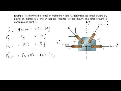
The review problem has four forces, labeled FA, FB, FC, and FD, acting at one particle.
Students begin by identifying the free-body diagram and deciding which component signs follow from each arrow’s direction.
The example uses the 60° and 45° directions to practice connecting diagram geometry to force components.

9:00 Assigning Signs to the 4 kN and Unknown Force Components

FA has magnitude 4 kN at 60° from the x-axis, giving positive components 4 cos 60° and 4 sin 60°.
FB and the 2 kN force FC act left, so each contributes a negative x-component even if its position on the page might suggest otherwise.
FD points down and right at 45°: its x-component is positive and its y-component is negative.
For a diagonal force, sine and cosine depend on which axis the reference angle touches; the component signs come from the arrow directions.

14:10 Solving the Four-Force Equilibrium Equations

The x-equilibrium equation is 4 cos 60° − FB − 2 + FD cos 45° = 0.
The y-equilibrium equation contains 4 sin 60° and the downward component −FD sin 45°, allowing FD to be found first.
Guidio reports approximately FD = 4.9 kN and FB = 3.46 kN.
Writing both equations before rearranging helps identify which one can directly solve an unknown.

17:10 Drawing the Free-Body Diagram for the Cable-Junction Example

The next problem asks for cable tensions AC and BC at joint C, with a 300 N angled load and a 200 N horizontal force shown.
Guidio isolates the joint and labels each cable force so the unknown tensions can be resolved into components.
The diagram provides 30° and 45° reference angles for the cable and applied-force directions.

20:10 Resolving Cable and Applied Loads into Components

For TBC, the chosen 30° reference gives a horizontal component TBC cos 30° and a vertical component TBC sin 30°.
For TAC, the x-component points left and is negative, while its y-component points upward and is positive.
The 200 N force acts left, and the 300 N force at 45° contributes positive x and negative y components.
The component equations must preserve both the reference-angle convention and each arrow’s direction.

22:42 Rearranging Two Cable Equations with Two Unknowns

Students work through the coupled equilibrium equations, which contain both TAC and TBC along with the known loads.
Guidio recommends isolating one unknown in one equation and substituting that expression into the other.
The algebra requires distributing trigonometric factors across terms; keeping the substitution in parentheses reduces sign errors.

31:40 Completing the Cable-Tension Algebra

Guidio groups known numerical terms before solving for one tension as a function of the other.
The example’s reported tension results are approximately 134 N and 110 N.
Students may retain exact sine and cosine values or convert them to decimals, provided each factor is applied consistently.
Guidio notes that the multi-step trigonometric manipulation is useful preparation for later dynamics problems, even if it is unusually lengthy for an exam.

38:40 Choosing the Solve Order for the Two-Particle Cable System

Students identify that the system requires separate free-body diagrams at points C and D.
The group chooses to analyze D first because the lamp’s mass determines its weight and makes one force known there.
At D, two unknown cable tensions can be solved with the two equilibrium equations; starting at C would leave three unknown tensions.
The tension in cable CD then links the D and C diagrams.

44:42 Finding Cable Forces Supporting the 20 kg Lamp

The lamp’s weight is calculated from 20 kg × 9.81 m/s², or 196.2 N.
At point D, Guidio resolves the cable forces using the 30° geometry and applies horizontal and vertical equilibrium.
The reported results are approximately FDE = 392 N and FCD = 339 N.
The known FCD tension is carried into the separate free-body diagram at point C.

49:15 Transferring FCD to Point C and Resolving the Cable Geometry

At point C, the cable directions use a 3–4–5 triangle for one cable and a 45° direction for the other.
The same cable force acts on each connected particle, but its arrow direction on the two free-body diagrams is opposite.
Guidio explains this direction change using tension: a rope pulls away from the particle at either end.
The discussion introduces tension and compression as physical interpretations of assumed force directions.

55:23 Solving the Remaining Tensions at Point C

The x-equilibrium equation combines the known 339 N FCD component with the x-components of FAC and FBC.
The y-equilibrium equation uses the 4/5 and 3/5 components of the 3–4–5 direction and the sine component of the 45° cable.
Solving the coupled equations gives approximately FBC = 274.62 N and FAC = 242 N.
Guidio recommends choosing the equation with fewer extra terms when isolating one unknown for substitution.

1:00:33 Setting Up the Final 100 N Equilibrium Example

The final problem gives P = 100 N and asks for the force in member AC.
The free-body diagram includes FAB and FAC, with 30° and 40° directions positioned relative to the particle.
Guidio uses the complementary 50° angle from the right-triangle geometry as an alternative way to describe the 40° direction.
Before calculation, students consider whether the assumed member-force arrows match the likely physical behavior.

1:07:46 Interpreting a Negative Result as Compression in AC

The x-equilibrium equation is used to express FAB in terms of FAC, then the expression is substituted into the y-equilibrium equation with the 100 N load.
The calculated FAC is about 92.16 N in magnitude, but its negative sign means the assumed tension direction was incorrect.
Guidio interprets the member as being in compression, not as having a physically negative force.
The final physical check is that the downward load pulls one member into tension while pushing the rigid member AC into compression.

Summary, takeaways, and chapters were generated by AI from the video's transcript and may contain errors. The video belongs to its creator, Bruno Guidio, PhD.