EDF9850_Example2_Part1
Overview
Lesa Hoffman demonstrates how to prepare the High School and Beyond data in R and fit a single-level baseline followed by an empty two-level random-intercept model using lme4. Across 7,185 students in 160 schools, the model estimates an intraclass correlation of about 0.18, shows why school clustering matters for inference and study planning, and illustrates how to explain school-level variation with a random-effect interval.
Key takeaways
- In the High School and Beyond example, an ICC1 of about 0.18 indicates substantial school-level dependence in student math scores and supports using a multilevel model.
- An average cluster size of about 45 combined with ICC1 of 0.18 produces a design effect near 9, so 7,185 clustered observations provide information comparable to roughly 800 independent observations.
- The empty multilevel model separates total variance near 47 into about 8.6 between-school variance and 39 within-school variance; adding a random intercept partitions variation rather than explaining it.
- The single-level intercept of about 12.7 is a student-weighted mean, while the multilevel intercept of about 12.637 represents the mean of school means and accounts for unequal school sizes.
- A random-effect interval of approximately 6.9 to 18.4 communicates the expected spread of school mean math scores in the outcome's original units, a different quantity from uncertainty around the fixed intercept.
- Keeping the analysis sample constant across models requires planning for missingness in all modeled variables, since each model otherwise may use a different set of students.
Chapters
- The example uses 7,185 students nested in 160 schools, with an average cluster size of about 45.
- R packages must be installed and loaded for each session; the pacman package streamlines this, while a working directory and helper-functions file support the analysis.
- Rows missing any modeled variables are excluded so sample sizes remain consistent across models; Hoffman notes that more advanced missing-data methods require a different modeling approach.
- School-level means are appended to the student data, and school size is recoded in 100-student units relative to a 1,000-student reference school.
- The empty single-level GLS model has a fixed intercept of about 12.7 and total math-score variance near 47, providing a comparison point for the multilevel model.
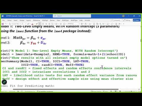
- The lme4 lmer model uses math as the outcome, a fixed intercept, and a random intercept grouped by school ID; Hoffman specifies REML estimation.
- The multilevel model partitions variance into about 8.6 between schools and 39 within schools, rather than explaining variance with predictors.
- The multilevel fixed intercept is about 12.637, the mean of school means, whereas the single-level intercept is the student-weighted mean.
- The intraclass correlation, ICC1, is about 0.18, meaning roughly 18% of math-score variance is associated with differences between schools.
- A likelihood-ratio test statistic near 900 greatly exceeds the 3.84 chi-square reference value Hoffman gives for the 0.05 level; variance-boundary testing uses a mixture p-value.
- With roughly 45 students per school and ICC1 of 0.18, the design effect is almost 9, reducing an effective sample size of 7,185 to roughly 800.
- For study planning, estimate a plausible ICC range from prior studies and combine it with the expected cluster size to assess how many participants clustering may require.
- ICC2 is described as high, indicating reliable school mean estimates given the number of students per school and the between-school variance.
- A random-effect interval translates the estimated school variation into the outcome scale: about 95% of school mean math scores are expected to fall between 6.9 and 18.4.
- That interval describes the spread of school means, unlike a fixed-effect confidence interval, which describes uncertainty in the estimated intercept across repeated samples.
- Hoffman asks students to finish Shiny apps 3 and 4 before the next class, focusing on the broad interpretation rather than exact answers.
Transcript excerpt
0:08 All right. Do you still have questions or is your hand just still up? >> I'm sorry. My hand is just >> I know it doesn't take it down like in in some versions of Zoom it automatically took it down after a while, but in others it didn't. So, I guess we're in that one. All right. So, what I've learned so far in this class is that shiny apps take more time than I predicted. Um, but they are useful for visualization. So, in the interest of time, what I'd like to do is go through two models. A single level model and your very first multi-level model that's empty. And we'll stop there. Um, apps three and four. I would say if uh we have time left in class, you're welcome to stay and work on them or else you can finish them on your own. Do not put a ton of time into answering the questions very specifically. like broad strokes is
0:55 what I'm looking for. Okay, it's it's designed as a tool to help you visualize things. It's not necessary to get like every single aspect of it correct. And this is useful for me planning what we will do in the upcoming weeks in terms of that. I only had two apps scheduled, so it looks like that's the most that one class could potentially have. I will work on revising the questions so that they're clearer and and less redundant as well, so we can keep that streamlined. But I do want to show you how to actually fit these models in software. So I am on example two there. If you haven't downloaded that yet, let me show you where that is. Get this back up here. So example, yeah, right here. Here's the PDF that
This is the start of the transcript. Save this video free for the whole transcript, searchable and time-coded.
In this course
Related notes
Summary, takeaways, and chapters were generated by AI from the video's transcript and may contain errors. The video belongs to its creator, Lesa Hoffman.