EDF9850_Lecture2_Part2
Overview
Lesa Hoffman explains how multilevel models use level-two school predictors, such as homework assigned and mixed-grade classrooms, to predict school mean language outcomes and reduce random-intercept variance. Using an example associated with Snijders and Bosker, she distinguishes fixed-effect tests and R-squared measures from likelihood-ratio tests of random effects, and explains why REML comparisons must hold fixed effects and observations constant.
Key takeaways
- A level-two predictor that is constant within each school has ICC 1, providing a diagnostic for identifying cluster-level variables when measurement levels are undocumented.
- School-level predictors explain between-school variance, not student-level residual variance directly; in the example, school predictors explained 3.6% of random-intercept variance and 6% of total language variance.
- Inference for school-level predictors must account for the number of schools, since a single-level regression can use student counts to produce misleadingly small standard errors.
- Use Wald tests for fixed slopes and likelihood-ratio tests for random-effect variances because variances are bounded at zero and violate the assumptions of a symmetric two-sided test.
- REML is preferred for estimating random-effect variances, especially with small samples, but valid REML comparisons require identical fixed effects and identical observations.
- Random effects partition outcome variability rather than explain it; report their variability with confidence intervals, and reserve variance-explained language for fixed predictors.
Chapters
- The example nests students, indexed by P, within schools, indexed by C, and uses school homework assignment and mixed-grade status to predict language outcomes.
- Homework is centered at 2, while mixed-grade status is coded 0 for no and 1 for yes.
- Because each level-two predictor is constant among students in the same school, it has no within-school variance and an ICC of 1.
- Adding school predictors to the unconditional random-intercept model predicts school means and estimates how much between-school variance remains.
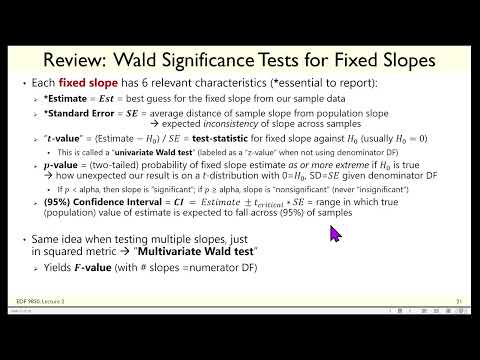
- A fixed-effect estimate is the sample slope, and its standard error measures how much that estimate would vary across repeated samples.
- For one slope, the estimate minus its null value, usually zero, divided by its standard error gives a t statistic, or a z statistic when degrees of freedom are not used.
- A p-value assesses how extreme the result would be if the null hypothesis were true; compare it with a prespecified alpha such as 0.05.
- Testing multiple slopes together uses a multivariate Wald test, commonly an F test; with one slope, t squared equals F, and z squared equals chi-square.
- After adding the two school predictors, the fixed intercept is 41.55, the expected language outcome for a school assigning two units of homework and not using mixed grades.
- Homework has a positive but nonsignificant slope, representing the change in school mean language for each additional homework unit relative to other schools.
- The mixed-grade slope is significantly negative, about two points lower for schools using mixed grades than for schools that do not.
- School predictors leave student-level residual variance near 62.2, while the random-intercept variance falls from about 17.88 to 17.2.
- Pseudo R-squared is calculated separately for each variance component as the proportional reduction from a model without the predictors to one with them; it can be negative.
- Homework and mixed-grade status explain about 3.6% of the random-intercept variance, meaning 3.6% of between-school mean differences.
- Total R-squared is the squared correlation between observed outcomes and predictions from fixed effects; the example explains about 6% of total language variance.
- Because the initial ICC is about 0.22, school-level predictors alone can explain at most that share of total variance; explaining student-level variation requires person-level predictors.
- A single-level regression without a random intercept gives different estimates, including a mixed-grade coefficient of about -1.5 rather than -2.
- Standard errors for school-level predictors should reflect the number of schools, not the much larger number of students; treating students as independent can understate uncertainty.
- Fixed effects can be evaluated with Wald tests, but deciding whether a random effect belongs in the model requires comparing model fit.
- A standard symmetric Wald test is unsuitable for testing a variance because variances cannot be negative, especially near the zero boundary.
- Maximum likelihood selects model parameters that make the observed data most likely; log-likelihoods add log densities across independent observations or, in multilevel models, clusters.
- A likelihood-ratio test compares nested models with and without a random effect using the difference in their log-likelihoods.
- The test statistic is the difference in -2 log-likelihood values, with degrees of freedom equal to the difference in parameter counts; a significant result indicates improved fit when adding the effect.
- For a variance tested at the zero boundary, the reference distribution is technically a mixture of zero and one degree of freedom, so the ordinary chi-square p-value can be halved.
- The school example retains an ICC of about 0.216 after adding homework and mixed-grade status; its random-intercept likelihood-ratio statistic is about 442, strongly supporting the two-level model.
- Maximum likelihood supports nested comparisons that differ in fixed effects, random effects, or both, but can underestimate level-two variances in small samples.
- REML more accurately estimates random-effect variances, but comparisons must keep fixed effects and the exact same observations in both models.
- Hoffman recommends describing random effects with confidence intervals and variability ranges rather than R-squared language; the lecture ends with a formative assessment that asks students to share walk-up music.
Transcript excerpt
0:01 Hello again. I am rehydrated and ready to keep talking. Picking up on slide 20 in lecture two describing how we add slopes for level two cluster specific predictors. So in general, level two predictors are between characteristics. In our cluster data context, level two predictors will be cluster specific variables that are constant over their persons. So, for example, in the Snyers and Bosser example data set here, we have level one students indicated by the P subscript nested in level two schools as the cluster, the C subscript. And we're going to examine whether language outcomes differ as a function of the amount of homework assigned at that school, which is a numeric variable that I centered at two given its range. So, that it would refer to about the average
0:48 school and whether or not the school has mixed grades in the same classroom in which zero is no and one is yes. So if we think about these two variables, these are cluster characteristics. Ask yourself for a moment, what would their ICC be? These are all between, no within variance because these scores will be constant for the kids from the same school. ICC for these level two predictors is going to be one. So that's a diagnostic that you can think about. If you're ever handed a data set and no one tells you at what level the variables are measured, interclass correlation will tell you. If you get an ICC of one back, that's a cluster characteristic. So if we start again with our empty model here, we have beta 0 C, which is our placeholder or backpack that then is
1:36 going to hold the fixed intercept gamma 00 plus the random intercept for school C that goes with it. This is what's
This is the start of the transcript. Save this video free for the whole transcript, searchable and time-coded.
In this course
Related notes
Summary, takeaways, and chapters were generated by AI from the video's transcript and may contain errors. The video belongs to its creator, Lesa Hoffman.