CS3130FS26Module4CVidProc
Overview
The lecture develops mergesort from its core operation, merging two ordered arrays, and explains how divide-and-conquer sorting can handle arrays too large for main memory by sorting manageable chunks and merging them. It derives merge comparison bounds and the Θ(n log₂ n) worst-case cost for power-of-two input sizes, then uses a median-selection example to show why partial merging can save comparisons and why algorithm solutions need explicit, logically justified comparison steps.
Key takeaways
- Mergesort can sort data larger than RAM by sorting memory-sized chunks independently and merging them incrementally, including writing completed portions out of memory.
- Merging arrays of sizes m and n takes at most m + n − 1 comparisons and at least min(m, n) comparisons, depending on when one input is exhausted.
- For evenly split input, mergesort satisfies T(n) = 2T(n/2) + n and has Θ(n log₂ n) worst-case comparison complexity.
- A rank-selection task does not require a complete merge: stopping when the target position is determined avoids comparisons for irrelevant later elements.
- Algorithm answers should explain the information gained from each comparison; a low comparison count without a justified sequence is not a verifiable solution.
Chapters
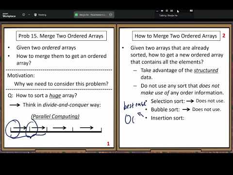
- The motivating case is an array larger than available RAM, with 64 GB given as an example limit.
- Divide the input into subarrays that fit in memory, sort each chunk with a normal sorting algorithm, then merge ordered chunks.
- When a combined run exceeds RAM, process portions of the runs, write merged output into place, and release processed portions from memory.
- Sorting independent chunks can be parallelized when multiple processors are available.
- Merging relies on the ordered property: the first unprocessed element of each sorted array is its current minimum.
- Selection sort does not exploit existing order, while bubble sort still performs comparisons even when the array is already sorted.
- Insertion sort benefits strongly from order, with best-case O(n) versus worst-case O(n²), motivating the merge approach.
- A single-element insertion step is a special case of merging two ordered arrays, where one array has size one.
- Mergesort generalizes insertion by combining two ordered arrays of multiple elements rather than an ordered run and one element.
- Split the original array as evenly as possible, repeatedly divide each part, and stop when every subarray contains one element.
- Merge adjacent ordered subarrays in successive rounds until a single ordered array remains.
- Balanced division avoids the poor worst-case behavior associated with highly unbalanced subproblems.
- Compare the first unprocessed elements of the two ordered subarrays; the smaller is the global minimum among the remaining elements.
- Place that smaller element next in the destination array, then compare it with the next candidate from its own subarray.
- Each comparison places one element in its final sorted position, continuing until one subarray is exhausted.
- Once one subarray is empty, the remaining elements of the other subarray can be copied without further comparisons.
- For subarrays of sizes m and n, the worst case takes m + n − 1 comparisons because only the final element can be placed without comparing.
- For two equal arrays of size k, the worst-case count is 2k − 1.
- The best case exhausts the shorter subarray as early as possible, requiring min(m, n) comparisons.
- The best- and worst-case counts differ because the merge can stop comparing as soon as either input runs out.
- For an array of n elements split evenly, the two recursive sorts contribute 2T(n/2).
- The merge step contributes at most n comparisons, giving T(n) = 2T(n/2) + n as an estimating recurrence.
- The recurrence uses base cases T(1) = 0 and T(2) = 1.
- The lecture drops the merge formula’s minus-one term to keep the asymptotic recurrence simple.
- Assume n = 2^k so repeated division by two produces integer-sized subproblems.
- Normalize the recurrence by 2^k and define G(k) = T(2^k)/2^k, yielding G(k) = G(k − 1) + 1.
- Starting from G(1) = 1/2 gives G(k) = k − 1/2, so T(2^k) = (k − 1/2)2^k.
- Substituting k = log₂ n gives a worst-case estimate on the order of n log₂ n; the general non-power-of-two proof is deferred to a recursion-tree method.
- A midterm problem asks for the sixth smallest value using two ordered arrays of five elements each plus a separate value x11.
- Fully merging the two five-element arrays can take 5 + 5 − 1 = 9 comparisons before considering x11.
- After a full merge, only the two middle candidates remain relevant, but comparing x11 with them adds two more comparisons.
- The key improvement is to stop the merge once the required sixth position is reached instead of completing all ten positions.
- A full merge of the two five-element arrays uses up to 9 comparisons.
- For the sixth-smallest rank among the resulting values and x11, rank-based elimination removes the four smallest and four largest merged positions.
- The two central candidates must each be compared with x11, adding two comparisons and bringing the described approach to 11.
- The example illustrates that sorting all the way to a complete merge performs work that the rank query does not require.
- During a merge, each comparison identifies the next element in sorted order, so the operation can stop once the sixth position is known.
- The lecture estimates six comparisons to reach that position, then two comparisons involving x11, for a total of eight.
- This partial-merge approach improves on the 11-comparison full-merge strategy.
- The instructor notes that eight is close to, but not equal to, the cited six-comparison best solution.
- Ordinary merging is presented as optimal when the combined input size is relatively small, with sizes around four to six given as examples.
- For larger combined sizes, including the example’s total of ten, a different method may use fewer comparisons for a selection task.
- The lecture distinguishes weak solutions, typically one comparison above the standard solution, from full-credit standard solutions and stronger solutions that save a comparison.
- Partial merging is useful for reaching a weak or sometimes standard result, but it does not automatically achieve the strongest comparison bound.
- For difficult homework problems, an answer with fewer comparisons is not sufficient if the comparison sequence and reasoning are missing.
- The instructor cautions against presenting an unexplained result that appears to come from enumerating thousands of cases with an AI tool.
- A strong solution should use elimination reasoning to reduce candidate cases and explain what each comparison establishes.
- Random comparisons or steps added to fit a precomputed answer do not demonstrate a valid algorithm; every comparison needs a coherent justification.
Transcript excerpt
0:00 So this is our sort number four, right? Yeah. >> Sort number four. First let's look at the basic idea here. We need to consider uh a basic problem. Merge two ordered arrays. The merge operation given two ordered arrays question how to merge them to get an ordered array. It's a very simple problem. Yeah. All right. Motivation. So why we need to study this question? Yeah.
0:50 So here let's consider a special situation. Although there are many reasons let's consider we need to solve a special problem. Sort a huge array. How large is it? Yeah. So the size of the array, think about the size of the array is extremely large that we cannot load the whole array into the main memory. That large
1:39 main memory we have a specific size, right? Yeah. 16 gigabytes, 32 gigabytes, 64 GB. So there is a specific size. In order to sort of our current algorithm, we need to load the whole array into the main memory then sort it. Yeah. But if our data size is extremely large, greater than 64 GB for example, so you do not have on your computer, you do not have that large
2:29 main memory, but you still you need to sort this array. Yeah. We we can do it. Yeah. So we we can apply some special technique to sort this huge array. So how to do it? Remember divide and conquer, right? So let us divide the this is the huge array. Divide this huge array into several sub subarrays not many subarrays. and make sure each subarray can be loaded into the main memory. Yeah. So that's pretty easy, right? Yeah. Make sure each subarray can be loaded into
3:18 the main memory and we can apply our normal sorting algorithm to sort it. Yeah. So
This is the start of the transcript. Save this video free for the whole transcript, searchable and time-coded.
In this course
Related notes
Summary, takeaways, and chapters were generated by AI from the video's transcript and may contain errors. The video belongs to its creator, DrHeUMSLTeaching.