CS3130FS26Module4AVidProc
Overview
The lecture develops insertion sort by growing a sorted prefix one element at a time, then analyzes its array-shifting implementation and its performance: best case Θ(n), average and worst cases Θ(n²). It applies comparison-sort lower bounds and binary insertion to show optimal sorting strategies for 3, 4, and 5 elements, with the five-element tournament method sorting in seven comparisons.
Key takeaways
- Insertion sort grows a sorted prefix one element at a time, taking Θ(n) comparisons on already sorted input but Θ(n²) on average and in the worst case.
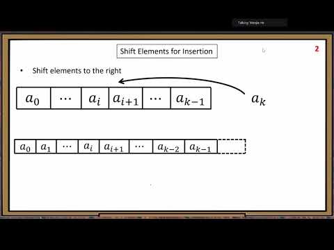
- Because array elements occupy consecutive memory locations, inserting into the middle requires shifting later elements even after the insertion position is determined.
- Insertion sort is particularly useful when data is nearly sorted, since already ordered regions require very little work.
- The worst-case comparison lower bound for comparison sorting is ceil(log₂(n!)); matching it proves optimality for the specific input size.
- The lecture's optimal small-array results are 3 comparisons for 3 elements, 5 for 4 elements, and 7 for 5 elements.
- Counting sort can avoid comparison-sort lower bounds when the input consists of integers from a sufficiently small range.
Chapters
- The module introduces divide and conquer, then contrasts it with a strategy that grows a solved problem by adding one element at a time.
- Selection sort and bubble sort have already been covered; insertion sort is introduced as a third sorting approach.
- The method starts with a one-element array, already sorted, and asks how to extend that solution while preserving order.
- Each step inserts the next element into the prefix that has already been sorted.
- For a two-element prefix, one comparison determines the order; inserting a third element takes one comparison in the best case or two in the worst.
- The general insertion step compares the new element with sorted elements from right to left, using the prefix's existing order.
- Insertion sort's core operation is placing a new element in the correct position in the sorted array.
- Array elements occupy consecutive memory locations, which allows an index to map to an address by calculation.
- When larger preceding values are found, they shift one position right; the new element is saved temporarily and placed in the gap.
- In the worst case, each newly added element moves past every element already in the sorted prefix.
- Across the full sort, the number of comparisons grows as 1 + 2 + … + (n−1), giving Θ(n²) worst-case work.
- The shifting assignments for an individual insertion can also grow linearly with the prefix length.
- For an already ascending array, each of the n−1 insertions needs only one comparison, so the best case is Θ(n).
- Under the lecture's linear distribution of insertion positions, an insertion uses about half the worst-case comparisons, yielding roughly n(n−1)/4 comparisons overall.
- The average case remains Θ(n²), despite the lower constant factor than the worst case.
- Insertion sort is a strong choice when most elements are already in order and only a few positions are disrupted.
- Ordered portions of the input can be processed close to the Θ(n) best case, while other common sorting algorithms may still perform more work.
- For general inputs, insertion sort's Θ(n²) average cost is usually outperformed by other sorting algorithms.
- The first two elements are ordered with one comparison, then the third is inserted with up to two more.
- The resulting three-comparison procedure is tested against the lower bound for comparison sorting.
- For n = 3, ceil(log₂(3!)) = ceil(log₂ 6) = 3, so the procedure is optimal.
- Any comparison sort needs at least ceil(log₂(n!)) comparisons in its worst case, because it must distinguish among n! possible input orders.
- The lower-bound claim applies specifically to comparison sorts, not to every possible sorting algorithm.
- Counting sort is presented as a non-comparison alternative for integer inputs drawn from a relatively small range.
- After sorting the first three elements in three comparisons, compare the fourth element with the middle element of the sorted prefix.
- That binary-insertion decision narrows its location to one of two pairs, requiring two further comparisons and five total.
- For n = 4, ceil(log₂(4!)) = ceil(log₂ 24) = 5, confirming that the method is optimal.
- Rather than repeatedly extending an insertion-sorted prefix, the five-element strategy starts by comparing the first four values in a tournament.
- Pairwise comparisons followed by a final comparison use three comparisons to establish a chain of ordered information.
- Four is convenient for the tournament structure because it is a power of two.
- In the example, X1 is compared with X2, X3 with X4, and then the pair winners X2 and X4 are compared.
- Assuming X4 wins the final comparison, the tournament provides the ordered chain X4, X2, X1, with X3 also placed relative to the comparisons.
- The next stage uses that known ordering to insert X5 efficiently rather than starting over.
- Binary insertion places X5 into the known chain with two additional comparisons, with cases depending on whether it belongs above or within the chain.
- The remaining out-of-order element is inserted using comparisons guided by the existing ordering; the lecture examines representative essential cases.
- The method uses seven comparisons in total: three in the tournament, two to place X5, and two to place the remaining element.
- For n = 5, ceil(log₂(5!)) = ceil(log₂ 120) = 7, so the seven-comparison procedure meets the comparison-sort lower bound.
- Finding the median of five is a related but different task; the lecture gives six comparisons as the target for that problem.
- The five-element sorting example combines tournament comparisons, known-order chains, and binary insertion.
Transcript excerpt
0:00 Start module four divide and conquer approach. Another very important uh problem solving approach. Uh we have used uh some of the ideas divide and conquer in module three. Uh but we need to learn more. Part A insertion sort right 8.1 in insertion operation. the same uh sorting problem but we need to use a different idea to solve it. So at this point uh we have learned selection sort bubble sort uh and this is the third one insertion sort right
0:55 here strategy. Yeah. So, so let's recall our problem solving strategy. So, we used many times before start with a simple case. Let us study a few simplest cases first to get some ideas, different understanding uh angles. All right. Then because eventually we need to work on the general problem size and the general case. So how do we go from special cases to the general case by growing the data
1:45 sizes gradually. Yeah. So that simple idea, right? Actually uh this idea it it is the opposite of divide and conquer. Divide we divide we make the problem sizes smaller. Here we can also understand the opposite way we grow. Yeah. Yeah. Yeah. All right. Grow. How much to grow? Every time increase the problem size by one add just one new element. Yeah. Divide. Every time you remember our first uh divine conquer case we divide the
2:36 problem by reducing the problem size by one. Yeah. Here the opposite way. Yeah. All right. how to connect two adjacent cases. So let's uh study simple examples. How to add every time we add one element after we solve the current problem when we move to the next sub problem we just add one new element to our data. That simple. All right, let me use a simple diagram
This is the start of the transcript. Save this video free for the whole transcript, searchable and time-coded.
In this course
Related notes
Summary, takeaways, and chapters were generated by AI from the video's transcript and may contain errors. The video belongs to its creator, DrHeUMSLTeaching.