CE 312 Lecture 38: Matrix Structural Analysis II, 1D Bar Element Derivation (2026.11.16)
Overview
Gregory Michaelson derives the 1D bar element stiffness matrix, K = (EA/L)[[1, -1], [-1, 1]], using unit-displacement cases and consistent force signs. He then explains how element matrices are assembled into a global system, how boundary conditions reduce it for solving displacements, and how the results recover reactions and member forces. A numerical example with three elements and a five-node, six-element spring assignment previews the Excel workflow.
Key takeaways
- The 1D bar element stiffness matrix is K = (EA/L)[[1, -1], [-1, 1]], derived by applying a unit displacement to each of the element's two degrees of freedom and recording the required end forces.
- Global assembly follows connectivity: place each 2×2 element matrix at the rows and columns for its connected nodes, and sum terms wherever multiple elements overlap.
- Boundary conditions turn the global structural equations into a solvable reduced system by excluding restrained degrees of freedom; a singular stiffness matrix can indicate insufficient restraints or instability.
- Once unknown displacements are solved, support reactions come from the full global stiffness equation, while each element's end forces come from its local stiffness matrix multiplied by its local displacement vector.
- A four-node bar system requires a 4×4 global stiffness matrix, while the assigned five-node spring network requires a 5×5 matrix, regardless of the fact that each individual element matrix is only 2×2.
Chapters
- Gregory Michaelson says only two weeks of class remain, with no homework due during the current week or the Monday after break.
- The project submittal must include the final MASTAN file with real loads and selected sections, computations, a reflection statement, and a complete CAD drawing submitted as a PDF.
- Friday's Lecture 40 is an optional project troubleshooting session without attendance or prepared lecture notes.
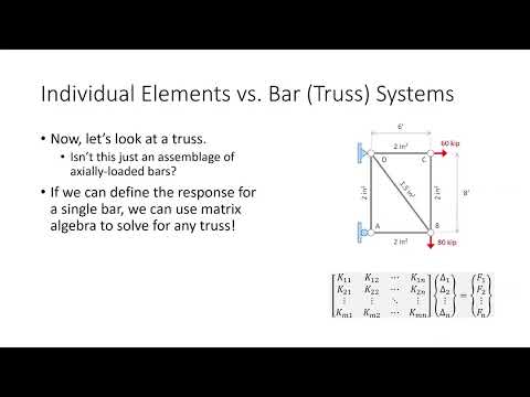
- Structural software performs preprocessing and postprocessing around a solve that returns support reactions, member responses, nodal displacements, and the deflected shape.
- An unstable model can produce a singular stiffness matrix; adequate boundary conditions are needed to make the system stable and the matrix invertible.
- For an axially loaded bar, F = (EA/L)δ, so EA/L is the axial stiffness and the force needed for a unit displacement.
- A 1D system has only horizontal forces and displacements, with members carrying tension or compression.
- Each node contributes a potential displacement degree of freedom; restrained nodes have known zero displacement, such as the three unknown displacements at B, C, and D when node A is fixed.
- A truss can be treated as an assemblage of bar elements, whose individual responses combine into a global stiffness matrix, displacement vector, and force vector.
- The bar element has two nodes, length L, constant Young's modulus E, and constant area A, with end displacements δ1 and δ2.
- Positive force and displacement directions are drawn to the right at both ends; leftward quantities are negative.
- The direct stiffness approach deforms the element in prescribed displacement cases and records the forces required to produce each case.
- For case 1, set δ1 = 1 and δ2 = 0; the bar shortens, requiring end forces +EA/L and -EA/L under the stated sign convention.
- For case 2, set δ1 = 0 and δ2 = 1; the bar lengthens, requiring end forces -EA/L and +EA/L.
- Using the two cases to identify the matrix columns gives K = (EA/L)[[1, -1], [-1, 1]], a symmetric element stiffness matrix.
- For a spring element, the spring constant replaces EA/L; the same direct-stiffness procedure applies.
- Write one element stiffness matrix per member, then assemble their terms into the global stiffness matrix according to node connectivity.
- Build the global force vector from applied loads and unknown support reactions, then apply boundary conditions by removing restrained degrees of freedom from the solve.
- Solve the reduced system for unknown displacements, using software such as Excel for matrix operations and inversion.
- Recover reactions from the full global equation and calculate each member's end forces by multiplying its element matrix by its element displacement vector.
- The upcoming example has four nodes, two support reactions, and only one horizontal equilibrium equation, so statics alone cannot determine the reactions.
- The global displacement vector is [0, δ2, δ3, 0]ᵀ, with zero displacements at the restrained end nodes.
- The force vector is [R1, 300, -125, R4]ᵀ, using rightward-positive signs for the loads and reactions.
- The example's element stiffness coefficients EA/L are 100, 200, and 100, calculated using inches rather than feet.
- Each 2×2 matrix uses its element's EA/L multiplied by [[1, -1], [-1, 1]].
- Element and degree-of-freedom codes identify where each local matrix contributes to the four-node global system.
- The three element matrices contribute to a 4×4 global stiffness matrix because the example contains four degrees of freedom.
- Place each local matrix term at the global row and column indices corresponding to its two connected nodes.
- When multiple elements contribute to the same global matrix position, add their stiffness terms rather than replacing one with another.
- A correctly assembled global stiffness matrix should be symmetric, and row or column sums provide an equilibrium-related check on assembly.
- The full example will be completed in Excel using the Lecture 39 template available on Blackboard.
- The homework system has five nodes, six spring elements, and two restrained nodes, so its global stiffness matrix is 5×5.
- For element K2, EA/L = 4 and the element connects nodes 1 and 4; its local matrix is [[4, -4], [-4, 4]], placed at those global node indices.
Transcript excerpt
0:04 Can you believe that? Uh >> other than finals, we only have two weeks left of class. That's it. Two weeks. So, all right, everybody. Um just a couple of housekeeping items. So, attendance is up to date. Uh as for the homework grading status, at least as of this morning, homework 8.3 was graded. Uh 8.4 four and 8.5 are still being graded. So, I think my my TA is going to try and chip away at a lot of that uh this week. Um, homework 9.1 was due today. I'm hoping that was a really quick assignment. That should have taken you no more than five minutes. Um, I have no more homework due this week. Okay. No more because I do have homework due like
0:54 on the Wednesday and Friday we come back, but I don't have any more homework due this week and no homework due the Monday we come back from break. Okay. So, um so I'm hoping that uh break truly is just that, a break at least in C312. Um I am going to go ahead and open up homework 9.2, but it's not due till Wednesday. You honestly could probably complete it this week if you wanted to, but I I want you more focused on the project submitt uh than anything because that is uh what is most critical path. Um again, I I've been sort of copying and pasting this uh sort of set of notes here on the slides for the past few weeks. Um I just want to make sure that everybody remembers all the items that they need to submit uh in their
1:41 submittal. They need their final mass tan file which contains the real loads and the final uh section selection. They need all their computations, the
This is the start of the transcript. Save this video free for the whole transcript, searchable and time-coded.
In this course
Related notes
Summary, takeaways, and chapters were generated by AI from the video's transcript and may contain errors. The video belongs to its creator, Gregory Michaelson.