Area between curves (Calc 1; Lecture 3-12; Fall 26)
Overview
Steve Butler develops area between curves from the definite-integral idea of adding thin slices, using top minus bottom for vertical slices and right minus left for horizontal slices. Examples show how to find intersections, split integrals when boundary curves change, and sometimes switch variables to simplify setup; the lecture also reviews substitution, including a trigonometric integral whose value is the quarter-circle area π/4.
Key takeaways
- For vertical slices, area is upper function minus lower function; for horizontal slices, it is right boundary minus left boundary.
- Split an area integral wherever the boundary curve changes, as in the first-quadrant region where the lower edge changes at x = 2.
- Choosing the integration direction can reduce the number of integrals: the region between √x and x − 2 needs two vertical integrals but only one horizontal integral.
- Definite-integral substitution requires changing both the differential and the bounds; the factor from dx must remain, as in the calculation that produces the target value −1.
- Some definite integrals are easier to interpret geometrically than to integrate symbolically: ∫₀¹√(1 − u²)du is the area π/4 of a unit-circle quadrant.
- Inverse-function relationships let vertical and horizontal slice areas complement each other, turning two complicated integrals into the area 10 of a 2-by-5 rectangle.
Chapters
- Steve Butler revisits a mean value theorem problem after correcting an error from the previous lecture.
- Setting f'(c) equal to the given average rate of change produces candidate values −1 and 13.
- Only a candidate inside the specified interval counts, so the valid answer is one point, not two.
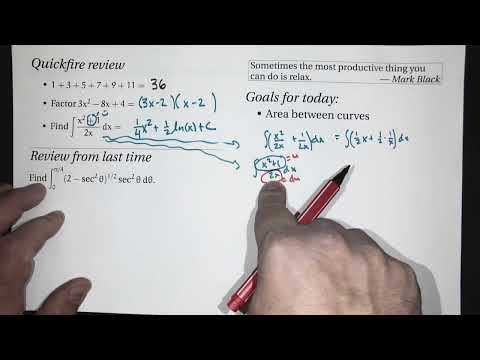
- The sum 1 + 3 + 5 + 7 + 9 + 11 is 36, illustrating the sequence of perfect squares.
- The quadratic 3x² − 8x + 4 factors as (3x − 2)(x − 2).
- For ∫(x² + 1)/(2x) dx, algebra separates the terms; setting u = x² + 1 does not work because the matching 2x is in the denominator.
- A definite integral from θ = 0 to π/4 uses u = tan θ, so du = sec²θ dθ and the bounds become 0 to 1.
- The transformed integral is ∫₀¹√(1 − u²) du, whose graph is the upper-right quarter of the unit circle.
- The area is one quarter of π·1², giving π/4; the method combines substitution, a trig identity, and geometric area.
- A target integral involving r(4x) is rewritten with u = 4x, converting its bounds to 2 and 4 and contributing a factor of 1/4.
- Other given integrals are similarly converted to integrals of r(u), with interval values including ∫₂⁶r(u)du = 10 and ∫₃⁶r(u)du = 12.
- Reversing the second interval and chaining 2→6→3→4 gives ∫₂⁴r(u)du = 10 − 12 − 2 = −4, so the target is −1.
- The supplied integral over 0 to 5 is unnecessary, illustrating that application problems may include more data than needed.
- For curves g(x) above f(x) on [a,b], the area is ∫ₐᵇ[g(x) − f(x)]dx.
- Each vertical rectangle has height g(x) − f(x) and width dx, so integration adds the slice areas.
- If the upper and lower curves switch, split the interval and set up separate integrals.
- Equating x² and x + 6 gives x² − x − 6 = 0, which factors to intersections at x = −2 and x = 3.
- Between those points, the line x + 6 is above the parabola x², so the area setup is ∫₋₂³[(x + 6) − x²]dx.
- Evaluating the definite integral gives an enclosed area of 125/6 square units.
- The first-quadrant region is bounded by y = √x, y = x − 2, and the coordinate axes, with key points (0,0), (2,0), and (4,2).
- For x from 0 to 2, the region lies between √x and the x-axis; from 2 to 4, it lies between √x and x − 2.
- The vertical-slice setup is ∫₀²√x dx + ∫₂⁴[√x − (x − 2)]dx, split where the lower boundary changes.
- Horizontal slices run from y = 0 to y = 2 and use width right minus left.
- Rewriting the boundaries as x = y + 2 for the line and x = y² for the parabola gives ∫₀²[(y + 2) − y²]dy.
- This single integral gives the same area as the two vertical integrals and is simpler because the left and right boundaries do not change.
- The curve y = √(x⁴ + 9) runs from (0,3) to (2,5), and solving for x gives x = ⁴√(y² − 9).
- A vertical-slice area under the curve and the complementary horizontal-slice area fit together to partition a rectangle with width 2 and height 5.
- Their sum is the rectangle's area, 2·5 = 10, even though the individual integrals are difficult to evaluate by antiderivatives.
Transcript excerpt
0:00 And I know what you're thinking. It's like Steve's going to say, "Oh, let's do our quickfire review." But no, I have to atone first. Last time I gave a problem and I goofed up. I wish I could blame the computer, but no, it was just human intelligence was the problem last time. So, so here is a better example of what I'm trying to get across. So, this should feel a little bit like deja vu. Hey, isn't this very similar to what we did last time? Yes, it is. But it'll work this time. find all the points satisfying the mean value theorem and uh as a reminder there's two mean value theorems will usually explicitly say which one we want so in this case we're talking mean value theorem for derivatives which says the
0:47 derivative frime of c minus f sorry frime of c is equal to f of b minus f of a over b minus a in other words your instantaneous rate of change is equal to your average rate of change and there's this extra assumption C is in the middle. Okay, so that's our mean value theorem. So now here's the function. Had to get a different function, different interval. So our function is x cubed - 18x^2 - 20x -5 up to 4 interval. and it goes ahead and says, "Hey, the average rate of change for this interval is 19." So, we don't have to compute that. So, good because I don't know if I'd want to compute something like 5 cubed. Yeah, sure. It's -125. But who knows that off
1:37 the top of their head? Nobody knows it off the top of their head. So, again, what do we want? Uh, oh, I wrote it down. We want the mean value theorem to
This is the start of the transcript. Save this video free for the whole transcript, searchable and time-coded.
In this course
Related notes
Summary, takeaways, and chapters were generated by AI from the video's transcript and may contain errors. The video belongs to its creator, Beard Meets Calculus.